Heuristic data-driven dynamic inertia estimation and multi-level stiffness optimization for servo motor parameter tuning

Karakaya, Mevlüt; Aküner, Mustafa Caner; Erken, Rabia İlknur; Ersoy, Sezgin

doi:10.21595/jmai.2026.26731

Journal of Mechatronics and Artificial Intelligence in Engineering

Browse Journal

Submit article

Published: September 27, 2026

Check for updates

Heuristic data-driven dynamic inertia estimation and multi-level stiffness optimization for servo motor parameter tuning

Mevlüt Karakaya¹

Mustafa Caner Aküner²

Rabia İlknur Erken³

Sezgin Ersoy⁴

^{1, 2, 3, 4}Department of Mechatronics Engineering, Marmara University, Istanbul, Turkey

Corresponding Authors:

Mevlüt Karakaya, Rabia İlknur Erken

Cite the article Download PDF

Article in Press

Downloads 0

Abstract

In this study, a data-driven heuristic approach with low computational cost and practical applicability is proposed to address the automatic parameter tuning problem in industrial servo motor systems. Experimental results obtained from 10,000 mm linear positioning tests demonstrate that the proposed method significantly reduces overshoot, settling time, and steady-state errors (MAE) compared to conventional manual tuning approaches through its dynamic inertia estimation and stiffness optimization modules. A odül advantage of the proposed approach is its ability to autonomously suppress external disturbances using only real-time velocity, position, and torque data without requiring complex mathematical models. The obtained results indicate that the proposed method provides a flexible, high-performance, and real-time capable automatic tuning solution for industrial servo applications.

1. Introduction

Servo motor systems are widely employed in motion control applications that require high precision, such as industrial robots, CNC machine tools, packaging lines, and automation equipment [1], [2]. Positioning accuracy, fast response, low tracking error, and stable operation are among the primary performance indicators of these systems [3], [4]. The proper tuning of controller parameters plays a critical role in achieving these performance objectives. In particular, the gain parameters and position-velocity loop settings used in proportional-integral-derivative (PID) and proportional-derivative (PD) controllers directly affect the dynamic behavior of the system [2], [4]. Improper parameter selection may lead to undesirable effects, including excessive overshoot, long settling times, vibration, high tracking errors, odüles system instability [2], [5]. Therefore, the effective and reliable tuning of controller gains in servo systems remains an important research topic in both academia and industry [4], [6].

In this context, numerous approaches have been developed in the odülese for servo system parameter tuning. Among the conventional tuning techniques, Ziegler-Nichols and Cohen-Coon-based methods are widely used due to their practical applicability for specific systems [7]. However, these methods generally require open-loop testing, rely on experimental procedures, and assume constant load conditions [4], [8]. In real industrial environments, load torque, friction characteristics, and mechanical coupling properties may vary over time [2], [9]. Consequently, conventional tuning methods often fail to maintain the desired level of performance under varying operating conditions [8], [9].

To overcome the limitations of conventional tuning techniques, model-based automatic tuning approaches have been developed. Techniques such as Model Reference Adaptive Control (MRAC) and Model Predictive Control (MPC) can achieve superior performance by explicitly considering system odüles [10], [11]. However, these methods are often of limited practical use in industrial applications due to their reliance on accurate mathematical models and their relatively high computational complexity [12], [13]. Furthermore, the presence of model uncertainties and external disturbances in real-world systems further restricts their applicability in industrial environments [10], [13]. Consequently, there is a growing need for more practical approaches that eliminate complex modeling requirements and make decisions directly based on data acquired from the system itself [13], [14]. In fact, the 10,000 mm stroke tests conducted in this study demonstrate that data-driven heuristic methods can not only improve reference-tracking accuracy but also significantly enhance system robustness against external disturbances [4].

In recent years, data-driven approaches based on fuzzy logic and artificial neural networks have also been investigated odüle automatic tuning of servo systems [15], [17]. These methods offer significant advantages in modeling nonlinear system behaviors and enabling adaptive decision-making capabilities. Nevertheless, issues such as membership function design, training data requirements, hyperparameter selection, and limited interpretability often complicate their deployment in industrial environments [15], [17]. In addition, these approaches are generally not directly compatible with the parameter configuration tables provided by servo drive manufacturers, which further limits their practical adoption in field applications.

At this point, the main challenge is that existing automatic tuning methods are often unable to adapt sufficiently fast to real-time load variations, while manufacturer-provided data resources are not effectively integrated into the decision-making process [4], [6]. In servo systems, variations in the load inertia ratio directly influence system odüles, particularly during acceleration and deceleration phases [9]. If controller gains are not adjusted appropriately in response to these variations, increased vibration, resonance phenomena, and tracking errors become inevitable [2], [3]. Furthermore, although many commercial servo drives provide predefined parameter tables for different mechanical configurations, these data are rarely utilized dynamically in conjunction with real-time measurements.

To address these challenges, this study proposes a heuristic data-driven method odüle automatic tuning of servo motor parameters. In the proposed approach, manufacturer-provided stiffness tables are integrated with real-time system data to support the tuning process. The dynamic inertia ratio is estimated online based on the torque–acceleration relationship, while an appropriate gain region is determined through a multi-level stiffness optimization strategy. Subsequently, a heuristic decision-making mechanism is employed to maintain a balance between oscillation tendency and tracking performance. In addition, a proportional scaling scheme is introduced to enable smooth transitions between gain levels, thereby ensuring more stable and continuous parameter updates. Through these features, the proposed method offers a practical, low-cost, and high-performance automatic tuning solution with strong potential for both theoretical investigations and industrial applications.

2. System architecture and methodology

2.1. Overall system structure

The proposed heuristic data-driven parameter estimation method is built upon a modular architecture capable of adapting to real-time operating conditions in servo motor systems. The developed framework is designed to continuously analyze feedback data acquired from the system and automatically determine appropriate control parameters. In this way, the performance of the servo system can be maintained under varying mechanical stiffness conditions and sudden changes in operating regimes [3], [4].

The overall algorithm consists of eight sequential and interconnected stages. In the first stage, real-time data are collected from the servo drive and feedback sensors. Subsequently, a preprocessing and filtering procedure is applied to reduce measurement noise and mitigate the effects of transient disturbances [5]. Using the filtered data, performance-related error metrics that characterize the system behavior are calculated [18], [19]. In the following stage, dynamic inertia estimation is performed based on the torque-acceleration relationship, enabling the online identification of load variations and their effects on the system odüles [9].

The estimated inertia information and calculated performance indicators are then utilized to determine an appropriate stiffness level. The control gains corresponding to the selected stiffness level are mapped to the system using manufacturer-provided parameter tables or predefined data maps. Subsequently, boundary checks and safety constraints are applied to ensure that the selected parameters do not violate system safety requirements. Finally, the updated position-loop and velocity-loop parameters are transmitted to the servo drive as the output of the tuning process [2], [4], [6].

The overall workflow of the proposed system can be summarized as follows:

Fig. 1System flowchart of the proposed method

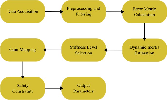
The proposed modular architecture enables each functional odüle to be developed and optimized independently, while also facilitating straightforward adaptation to different servo drive manufacturers and application-specific requirements

2.2. Data acquisition and preprocessing

The performance of the proposed method is directly dependent on the accuracy and quality of the feedback data acquired from the system. Therefore, operational data obtained from the servo drive are continuously monitored at a predefined sampling frequency [3], [5]. In practical applications, the sampling frequency is selected by considering both the communication capability of the drive and the available processing resources. While a higher sampling frequency enables more accurate detection of rapid system variations, it also increases the computational burden. Consequently, a balance must be maintained between control performance and computational cost [3], [4].

A sliding-window approach is employed for data analysis [13], [14]. During each computation cycle, a data window consisting of a fixed number of samples is evaluated. In this study, the window size is defined as $N =$ 1000 samples. This approach enables both short-term transient effects and steady-state behavioral components to be analyzed simultaneously, thereby providing a more robust and stable decision-making mechanism [13].

These signals are utilized for tracking performance evaluation, dynamic inertia estimation, and the determination of an appropriate gain level [4], [6]. In industrial environments, measurement signals are often affected by electrical noise, mechanical vibrations, sensor resolution limitations, and friction-induced irregularities. To prevent these disturbances from adversely influencing the decision-making process, the raw data are subjected to a preprocessing stage. In this context, low-pass filtering and moving-average techniques are employed [5]. While the low-pass filter suppresses high-frequency noise components, the moving-average method reduces the impact of short-term fluctuations and transient variations. Particularly in low-speed operating regions, friction effects and stick-slip phenomena may cause significant fluctuations in velocity and torque signals [2]. Through the filtering process, these effects are mitigated, resulting in more reliable acceleration and torque estimations [9]. Consequently, the accuracy of the error analysis and inertia estimation procedures performed in the subsequent stages is significantly improved [18], [19].

Table 1Fundamental signals acquired from the servo system

Signal	Description
CmdVel	Reference velocity command
CmdPos	Reference position command
ActPos	Actual position feedback
CmdTrq	Torque command
ActTrq	Measured / estimated torque

3. Proposed mathematical framework

This section presents the mathematical framework developed for the heuristic data-driven automatic tuning of servo motor parameters. The proposed method consists of five main stages: the calculation of system performance indicators, online estimation of the dynamic inertia ratio, multi-level stiffness optimization, gain parameter mapping, and the application of safety constraints. Through these processes, the servo system is intended to maintain both stable operation and high performance under varying load conditions.

3.1. Performance metric: mean absolute error (MAE)

To quantitatively evaluate the velocity and position tracking performance of the servo system, the Mean Absolute Error (MAE) metric is employed [18], [19]. For the velocity control loop, the MAE is defined as follows:

1

{M A E}_{v e l} = \frac{1}{N} \sum_{t = 1}^{N} |c m d V e l_{t} - a c t V e l_{t}| .

Similarly, for the position control loop, the error metric is defined as:

2

{M A E}_{p o s} = \frac{1}{N} \sum_{t = 1}^{N} |c m d P o s_{t} - a c t P o s_{t}|,

where, $N$ denotes the total number of samples within the analysis window. Higher MAE values indicate that the system is unable to track the reference signal with sufficient accuracy [18], [19].

Within the proposed decision-making framework, the system is classified as having insufficient stiffness or inadequate dynamic response characteristics when the following condition is satisfied:

3

M A E_{v e l} > 5.0 o r M A E_{p o s} > 2.0 .

3.2. Dynamic inertia ratio estimation

To effectively monitor the influence of load variations in servo systems, the inertia ratio is estimated online. In the first step, the acceleration is calculated from the actual velocity signal using a numerical differentiation method [3], [9]:

4

a (t) = a c t V e l (t) \approx \frac{∆ a c t V e l}{∆ t} .

To capture periods characterized by significant dynamic activity, only samples belonging to the upper 20th percentile of the acceleration distribution are selected:

Ahigh = $\{t∣ a (t) > p e r c e n t i l e 80 (a)\}$ .

Within the selected regions, the actual torque and commanded torque values are compared to calculate the dynamic torque factor [4], [9]:

5

T o r g u e F a c t o r = \frac{\frac{1}{|A_{h i g h}|} \sum_{t \in A_{h i g h}} |a c t T r q_{t}|}{\frac{1}{|A_{h i g h}|} \sum_{t \in A_{h i g h}} |c m d T r q_{t}|} .

Subsequently, the current inertia ratio is updated according to the following bounded update rule:

6

N e w I n e r t i a = C u r r e n t I n e r t i a \times m a x (0.5, m i n (T o r q u e F a c t o r, 1.5)) .

The imposed constraints prevent sudden parameter fluctuations, thereby enhancing system stability and ensuring smoother adaptation to changing operating conditions [3], [5].

3.3. Stiffness level optimization algorithm

To ensure that the servo system operates at an appropriate stiffness level, a multi-criteria heuristic decision-making mechanism is proposed. First, the zero-crossing rate of the velocity error signal is analyzed. A high zero-crossing rate indicates the presence of high-frequency oscillations within the system [2], [3]. If:

7

z e r o c r o s s i n g r a t e (v e l e r r o r) > 0.10 .

The system is considered to exhibit oscillatory behavior, and the stiffness level is reduced by two levels.

Conversely, if:

8

M A E_{v e l} > 5.0 o r M A E_{p o s} > 2.0 .

The system is regarded as having an insufficient dynamic response, and the stiffness level is increased by two levels [6], [18], [19].

If neither condition is satisfied, the current stiffness level is maintained. In this manner, the system is adaptively tuned to achieve a balance between oscillation suppression and tracking accuracy [2], [4].

3.4. Gain parameter mapping

For the selected stiffness level, $R \in$ [1, 20] the control gains are mapped using manufacturer-provided tuning data. This mapping process can be expressed by the following function:

9

[P o s G a i n 1, S p d G a i n 1, S p d I n t 1, T r q F i l t 1] = F t a b l e (R),

where, $F_{t a b l e}$ denotes the parameter mapping function derived from the manufacturer’s technical documentation and implemented using piecewise linear interpolation. This approach enables the selection of near-optimal drive parameters for each stiffness level [4], [6].

3.5. Secondary gain scaling (Gain 2 calculation)

To proportionally transfer changes occurring in the primary gain group to the secondary gain group, a scaling factor is introduced. This approach is based on the principle of maintaining proportional relationships between control parameters in order to ensure smooth and stable parameter transitions within the control system [3], [5]:

10

λ_{p o s} = \frac{N e w P o s G a i n 1}{O l d P o s G a i n 1} .

Using this scaling factor, the secondary gain value is updated as follows:

11

N e w p o s g a i n 2 = O l d P o s G a i n 2 \times λ_{p o s} .

Similarly, to ensure a smoother transition of the velocity integral parameter, the following scaling relationship is applied:

12

{N e w S p d I n t}_{2} = 1.5 \times {N e w S p d I n t}_{1} .

This relationship is employed to update the corresponding gain parameter. As a result, instability and oscillatory tendencies that may arise from abrupt gain variations during parameter updates are effectively reduced [2], [4].

3.6. Safety and filtering constraints

To ensure the safe operation of the proposed algorithm in industrial applications, additional constraints are imposed. First, the standard deviation of the torque error signal is calculated [3], [5]:

13

σ_{t r q} = \sqrt{\frac{1}{N}} \sum {(c m d T r q_{i} - a c t T r q_{i} - μ)}^{2} .

If: $σ_{t r q} >$ 3.0 the torque filter gain is increased to suppress high-frequency noise components [5].

In addition, an acceleration limit check is performed:

14

\max (|a (t)|) > 50 .

If this condition is satisfied, the position filter level is increased to prevent sudden mechanical stresses and excessive dynamic loading [2], [9].

Through this safety layer, the proposed method provides not only performance-oriented tuning but also a reliable and practically deployable automatic tuning framework suitable for real-world industrial environments [4].

4. Experimental verification

In this section, the performance of the proposed heuristic-data-driven auto-tuning algorithm is validated across two distinct scenarios, based on a specific linear positioning task of 10,000 mm for the servo motor. The primary objective is to demonstrate, via graphical data, the efficacy of the calculated parameters in attenuating tracking errors and transient disturbances within the system.

4.1. Experimental setup

To test the industrial validity of the proposed algorithm, an experimental data acquisition setup was established utilizing a 400 W AC servo motor with a rated torque of 1.27 Nm and a nominal speed of 3000 rpm. During the data collection phase, commanded and actual speed and position data were extracted from the motor drive at a sampling period of 100 ms and subsequently stored in a relational database for offline analysis.

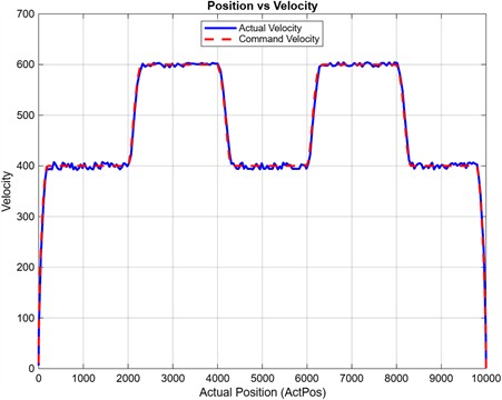
The computational optimization was carried out in the MATLAB environment. To evaluate the performance of the proposed algorithm under different operating conditions, the positioning of the motor from the starting point to the target of 10,000 mm was executed across two distinct scenarios. In the first scenario, the system was configured to reach the target position with a constant peak velocity. In the second scenario, a variable-speed profile – where velocity commands were altered at specific positions throughout the motion – was applied to assess the algorithm's capability to adapt to dynamic reference changes. To enable the algorithm to analyze the baseline state, the factory-default parameter set actively running on the drive was initially fed into the system as the initial condition; Data 1 and Data 3 were recorded to reflect the pre-optimization baseline for the constant-speed and variable-speed motions, respectively. Subsequently, the optimized parameters generated by the algorithm were uploaded to the drive, and the identical 10,000 mm motion profiles were repeated, yielding Data 2 for the constant-speed optimization and Data 4 for the variable-speed optimization. Consequently, the pre- and post-optimization results were comparatively analyzed across a total of four distinct datasets.

In this study, two distinct motion scenarios were formulated to validate the performance of the proposed dynamic proportional tuning algorithm under both baseline and complex field conditions. The first scenario, a constant-speed positioning profile, was selected as a benchmark test to evaluate the system's fundamental reference-tracking accuracy, its capacity to minimize steady-state error, and its success in attenuating standard mechanical friction effects encountered over a long distance (10,000 mm). Conversely, the variable-speed motion profile designated as the second scenario aims to test the algorithm’s robustness and adaptability against dynamic inertia variations frequently encountered in industrial fields. By altering the target speed during motion (transitions between 400 and 600 units), the study analyzes how the algorithm autonomously suppresses asymmetric torque losses occurring along acceleration/deceleration ramps, as well as mechanical resonance triggered particularly at high rotational speeds. This two-stage validation approach is specifically designed to demonstrate that the developed heuristic method delivers reliable control not only under stable operating conditions but also during aggressive operations characterized by abrupt reference variations.

4.2. Performance comparison and graphical analysis

The performance evaluation of the system was conducted through Mean Absolute Error (MAE) metrics, which reflect the overall tracking success throughout the target positioning, alongside the visual analysis of speed-position graphs. To compare the pre- and post-optimization performance, the following error formulation was taken as a basis. First, the instantaneous speed error $e_{v}$ is defined as the difference between the commanded speed $c m d V e l$ and the actual speed $a c t V e l$ .

The Mean Absolute Error (MAE), which measures the overall performance of the system, is formulated as follows, where $N$ represents the total number of samples:

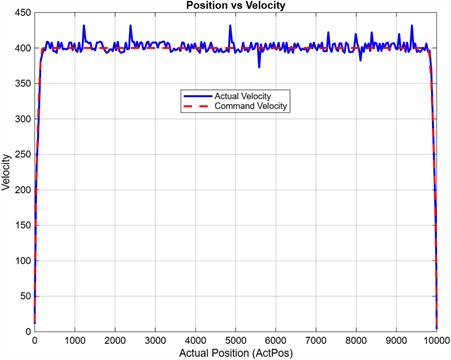
Scenario 1 – Pre-Optimization State (Default Parameters – Data 1): When analyzing the velocity-position graph of the constant-speed motion prior to the activation of the algorithm, it is observed that although the commanded velocity is set to 400 units, the actual velocity curve fails to track this reference value stably. Rather than producing a steady-state error within a specific band, the system is found to generate continuous, high-amplitude fluctuations around the reference velocity throughout the motion. In particular, sudden spikes where the actual velocity climbs up to 430 units are observed around positions of 1,000, 2,000, 5,000, and 9,500 mm, while sharp drops down to 380 units are recorded within the 6,000 and 8,000 mm bands. This behavior demonstrates that the factory-default rigidity levels and filtering parameters are insufficient to cope with external disturbances, friction variations, or mechanical resonance, thereby causing the system’s velocity loop to suffer from significant oscillation.

Table 2Factory-default controller parameters for Scenario 1 (Data 1)

Parameters name	Value
Inertia ratio	100
Position loop gain 1	50
Speed loop gain 1	75
Speed loop integral 1	50
Torque filter 1	5
Position loop gain 2	30
Speed loop gain 2	50
Speed loop integral 2	50
Torque filter 2	5
Position cmd filter	0

Fig. 2Velocity-position profile under factory-default parameters

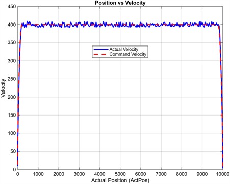
Scenario 1 – Post-Optimization State (Proposed Method – Data 2): The Data 2 graph, obtained after applying the new gains and filtering parameters calculated by the proposed heuristic algorithm to the system, demonstrates a significant and critical improvement in control performance. The actual velocity curve tightly locks onto the 400-unit commanded velocity reference, and the high-amplitude oscillations observed prior to optimization are substantially narrowed. The most pronounced improvement is manifest in the attenuation of disturbances; the aggressive velocity spikes and drops that reached up to 430 and 380 units in Data 1 are successfully suppressed following the algorithm's dynamic rigidity intervention. The actual velocity profile is confined within a narrow band of approximately ±5 units, corresponding to the limits of hardware mechanical tolerances and sensor noise, thereby maintaining stability and tracking the reference velocity with high precision throughout the 10,000 mm displacement.

Table 3Optimized controller parameters for Scenario 1 (Data 2)

Parameters name	Value
Inertia ratio	90
Position loop gain 1	40
Speed loop gain 1	60
Speed loop integral 1	69
Torque filter 1	8
Position loop gain 2	27
Speed loop gain 2	45
Speed loop integral 2	61
Torque filter 2	7
Position cmd filter	1

Fig. 3Velocity-position profile achieved by the proposed algorithm

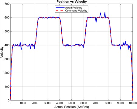
Scenario 2 – Pre-Optimization State (Variable-Speed Profile, Default Parameters – Data 3): When analyzing the graph corresponding to the factory-default settings of the second scenario (Data 3), which was formulated to test the algorithm's performance against dynamic reference variations, it is observed that the system exhibits severe stability issues while tracking the variable speed commands of 400 and 600 units. In addition to the fluctuations noted in the constant-speed first scenario, the control performance degrades dramatically in high-speed regions where the reference velocity escalates to 600 units.

Table 4Factory-default controller parameters for Scenario 2 (Data 3)

Parameters name	Value
Inertia ratio	100
Position loop gain 1	50
Speed loop gain 1	75
Speed loop integral 1	50
Torque filter 1	5
Position loop gain 2	30
Speed loop gain 2	50
Speed loop integral 2	50
Torque filter 2	5
Position cmd filter	0

Within the 400-unit segments of the motion-specifically along the 1,000-2,000 mm and 8,500-9,500 mm intervals-the actual velocity oscillates between 370 and 430 units. Crucially, the system significantly loses its stability during the second high-speed plateau of 600 units, particularly between 7,000 and 8,000 mm. In this region, the actual velocity is found to experience a sharp drop down to 560 units, immediately followed by aggressive spikes reaching the 630-640 unit bands, which generate resonant responses. This behavior demonstrates that the standard parameter set fails to respond rapidly to variable inertia profiles along acceleration/deceleration ramps and leaves the system highly vulnerable to mechanical noise at higher operational speeds.

Fig. 4Velocity-position profile under variable-speed commands with factory-default parameters

Scenario 2 – Post-Optimization State (Variable-Speed Profile, Proposed Method – Data 4): Analysis of the Data 4 graph, which highlights the success of the proposed heuristic algorithm under dynamic reference variations, clearly demonstrates that the optimization process elevates system stability to an advanced level across both speed bands (400 and 600 units). The severe resonant responses observed prior to optimization (Data 3) – which spanned between 560 and 640 units, particularly within the 600-unit high-speed plateau between 7,000 and 8,000 mm – are successfully suppressed owing to the algorithm's dynamic inertia estimation and torque command filtering.

Table 5Optimized controller parameters for Scenario 2 (Data 4)

Parameters name	Value
Inertia ratio	90
Position loop gain 1	40
Speed loop gain 1	60
Speed loop integral 1	65
Torque filter 1	9
Position loop gain 2	27
Speed loop gain 2	45
Speed loop integral 2	58
Torque filter 2	8
Position cmd filter	2

The actual velocity curve tightly locks onto the commanded velocity within a very narrow hardware tolerance band at both the 400-unit baseline speed and the 600-unit peak speed regions. Furthermore, the adaptation capability of the system is significantly enhanced along the acceleration ramps climbing from 400 to 600 units and the deceleration ramps dropping from 600 to 400 units, completing the transitions stably without any pronounced overshoot or oscillation. These findings confirm that the algorithm delivers an exceptionally high attenuation performance not only under static conditions but also against abrupt inertia changes and mechanical disturbances induced by variable-speed profiles.

When evaluating the optimized parameters computed by the algorithm for Scenario 1 (constant speed) and Scenario 2 (variable speed), it is observed that the inertia ratio (90), which dictates the fundamental stiffness of the system, alongside the primary/secondary position and speed loop gains, remain entirely identical across both scenarios. Conversely, the algorithm is found to perform precise fine-tuning on the integral time constants and filtering parameters in response to the dynamic disturbances induced by the variable-speed motion. In the second scenario, to enable a more rapid system response to dynamic reference variations, the primary speed loop integral time (Speed Loop Integral 1) is tightened by reducing it from 69 to 65, while the secondary integral time is decreased from 61 to 58. Simultaneously, to suppress mechanical noises that might arise along acceleration/deceleration ramps at varying velocities, the torque command filters (Torque Filter 1 and 2) are incremented by one unit, reaching values of 9 and 8, respectively, while the position command filter (Position Cmd Filter) is raised from 1 to 2. This behavior reveals that while maintaining core gain stability, the proposed algorithm achieves autonomous adaptation against variable-speed profiles primarily through the adjustment of integral time constants and specific noise-attenuation filters.

Fig. 5Velocity-position profile achieved by the proposed algorithm under variable-speed commands

4.3. Effects of dynamic adaptation

At the core of these achieved graphical improvements lies a dynamic and proportional computational model that abandons conventional fixed-rigidity tables. Rather than relying solely on position or velocity deviations, the algorithm performs an autonomous state diagnosis by computing the mean absolute error of the system and the oscillation ratio within the velocity loop.

Oscillation-Dominant Regime: In the presence of high-frequency oscillations and oscillation ratios exceeding 10 %, as observed in Data 1, the algorithm avoids excessively increasing the filters to prevent phase lag and sawtooth fluctuations. Instead, it scales down the position/velocity gains proportionally by a maximum of 20 % and extends the integral time constant by 30 % to pull the system back into the stability band. This dynamic intervention is calculated under the condition of OscRatio > 0.10 utilizing the following constrained functions:

15

g_{f a c t o r} = m a x (0.80, 1.0 - (O s c R a t i o - 0.10) \times 1.0),

16

i_{f a c t o r} = m i n (1.30, 1.0 + (O s c R a t i o - 0.10) \times 2.0) .

To guarantee system safety, the increase in the torque command filter for noise-mitigation purposes is restricted to a narrow band with a maximum limit of +2 units, without being explicitly incorporated into the main formulations.

Tracking-Error-Dominant Regime: In the presence of the sags and asymmetric velocity losses observed in variable-speed profiles – specifically under the condition of $M A E >$ 2.0 (as seen in Data 3) – the system rigidity is dynamically increased. The algorithm scales up the gains and tightens the integral time constant to enable the motor to lock onto the commanded velocity more aggressively. This stiffening process is executed using the following equations, which are linearly dependent on the error severity:

17

g_{f a c t o r} = m i n (1.30, 1.0 + (M A E - 2.0) \times 0.02),

18

i_{f a c t o r} = m a x (0.70, 1.0 - (M A E - 2.0) \times 0.02) .

Simultaneously, the instance where the actual velocity experiences a sudden drop while the commanded velocity remains high is detected via asymmetry analysis; subsequently, the inertia ratio is scaled up by a maximum of 20 % based on the combined feedback of the current inertia ratio, MAE, and asymmetry severity.

5. Discussion

In this section, in light of the findings obtained from the experimental studies, the advantages, current limitations, and field applicability potential of the proposed data-driven heuristic auto-tuning method are evaluated from the perspectives of control theory and industrial practices.

5.1. Advantages of the proposed method

The results of the executed linear stroke and variable-speed profile tests confirm that the proposed data-driven method not only enhances reference-tracking accuracy but also strengthens system robustness against disturbances. The foremost advantage of this approach lies in its utilization of a continuous and proportional mathematical model, rather than the static rigidity/tuning look-up tables conventionally employed in the industry.

Unlike conventional PID tuning methods frequently encountered in the literature, which induce oscillations by generating phase lag due to over-filtering, the proposed algorithm performs fine-tuning utilizing Mean Absolute Error (MAE) and standard deviation data. Dynamically updating the inertia ratio directly through asymmetric sags optimizes the starting and stopping torque under variable-speed references characterized by heavy load variations. Furthermore, compared to architectures that demand high computational power, such as complex model reference adaptive control (MRAC), this framework operates solely on Commanded Velocity (CmdVel) and Actual Velocity (ActVel) data, making it highly suitable for execution on standard PLCs and edge processors with low cycle times.

5.2. Limitations and algorithmic constraints

Despite the successful results obtained, certain limitations stemming from the hardware and mathematical structure of the system exist. The detection of asymmetric sags and the dynamic estimation of the inertia ratio fundamentally rely on taking the numerical derivative of the velocity data with respect to time $(a (t) \approx Δ a c t V e l / Δ t) .$ Although the 100-millisecond sampling period ( $T_{s} =$ 0.1 s)utilized in the experimental setup is sufficient to capture macro-level acceleration variations and asymmetric dropouts, the derivative computation carries the risk of inducing numerical instability in environments characterized by high-frequency mechanical noise. The probability of the algorithm missing instantaneous resonances on the order of microseconds is a natural consequence of this sampling frequency.

Another constraint emerges when the algorithm maximizes the dynamic gain factors $(g_{f a c t o r}) .$ In order to minimize the steady-state error of the system and reduce the MAE value, the algorithm may drive the gain values close to the hardware upper bounds – such as the 400 band – which can induce high-frequency oscillations in the motor shaft and mechanical transmission components. Although the algorithm analyzes high-frequency noise on the actual velocity via the velocity standard deviation $σ_{v e l}$ and intervenes in the torque command filters, this filter increment is strictly bounded for safety considerations. While this restriction is critical to preclude phase lag, hardware inadequacies due to encoder resolution limits can manifest when the natural frequency boundaries of the mechanical system are transcended.

5.3. Industrial applicability

Although data collection within the scope of this research was logged to the database at 100 ms intervals and the optimization processes were executed offline in the MATLAB environment, the core architecture of the algorithm is inherently suitable for direct embedding into industrial hardware. Because the decision-making mechanism of the algorithm relies on MAE and standard deviation-based statistical filters, simple algebraic equations, proportional factors, and bounded conditional blocks – rather than matrix computations or complex look-up tables that demand heavy computational loads – its computational cost is remarkably low. Consequently, it can be deployed on standard PLCs or motion controllers utilizing languages such as Structured Text (ST), C++, or Python with execution cycle times on the order of microseconds. Especially in long-stroke linear axis setups, such as 10,000 mm systems, this data-driven autonomous approach is anticipated to substantially reduce commissioning and periodic maintenance times.

6. Conclusions

In this study, a data-driven heuristic algorithm is proposed, offering a practical and computationally lightweight solution to the auto-tuning problem encountered in industrial servo motor systems. Based on the results of the executed 10,000 mm linear constant and variable-speed positioning tests, it is demonstrated that the algorithm's dynamic inertia estimation, proportional gain, and filter optimization modules significantly reduce the overshoot ratio, oscillations, and steady-state errors compared to standard factory parameters. The capacity of the method to autonomously attenuate external disturbances by processing primarily the commanded and actual velocity data obtained from the drive – without requiring complex mathematical models – highlights its industrial added value and real-time applicability.

In future works, it is planned to further optimize the existing heuristic decision tree and proportional factor limits utilizing machine learning techniques such as reinforcement learning. To demonstrate the flexibility of the algorithm, the implementation is intended to be extended from a single-axis motion structure to multi-axis synchronization systems. Furthermore, performing data fusion with external vibration or shock sensors is aimed at the early detection of high-frequency mechanical resonances.

Furthermore, it is aimed to transition the data analysis architecture – which is currently logged to the database at 100 ms intervals and executed offline – into a directly deployable edge computing framework on industrial PLC systems. The dynamic inertia ratio variations, attenuated mechanical resonance frequencies, and high-frequency velocity fluctuations $σ_{v e l}$ continuously monitored by the algorithm throughout the operation are envisioned to be processed within a Digital Twin infrastructure utilizing Deep Learning-based time-series analysis, rather than merely for instantaneous parameter adjustments. This integration will establish a comprehensive research foundation for monitoring the mechanical wear profiles of servo motors and transmission components, as well as for conducting Remaining Useful Life (RUL) estimations.

References

J. J. Craig, “Introduction to robotics: mechanics and control,” IEEE Transactions on Automatic Control, Vol. 32, No. 5, pp. 463–464, 2005, https://doi.org/10.1109/tac.1987.1104613

Publisher
P. Wang, T. Feng, C. Song, J. Li, and S. X. Yang, “A study of the stability of an industrial robot servo system: PID control based on a hybrid sparrow optimization algorithm,” Actuators, Vol. 14, No. 2, p. 49, Jan. 2025, https://doi.org/10.3390/act14020049

Publisher
N. S. Nise, “Control systems engineering,” in Automation in Textile Machinery, Hoboken, NJ, USA: John Wiley & Sons, 2019, pp. 1–35, https://doi.org/10.1201/9781315155333-1

Publisher
L. Kong, J. Wang, H. Hu, X. Dong, and B. Liu, “A novel tuning method for PID controller and its application in permanent magnet synchronous motor servo systems,” Actuators, Vol. 15, No. 3, p. 131, Feb. 2026, https://doi.org/10.3390/act15030131

Publisher
R. C. Dorf and R. H. Bishop, Modern control systems. Upper Saddle River, NJ, USA: Pearson, 2011.

Search CrossRef
K. Jinai, Y. Tsunoda, N. Kawaguchi, O. Arrieta, and T. Sato, “Data-driven design of fractional-order PID controllers: optimization of robust servo-regulator performance,” Journal of Robotics and Mechatronics, Vol. 37, No. 3, pp. 688–699, Jun. 2025, https://doi.org/10.20965/jrm.2025.p0688

Publisher
J. G. Ziegler and N. B. Nichols, “Optimum settings for automatic controllers,” Transactions of the ASME, Vol. 64, No. 8, pp. 759–765, 1942, https://doi.org/10.1115/1.2899060

Publisher
H. O. Bansal, R. Sharma, and P. R. Shreeraman, “PID controller tuning techniques: a review,” Journal of Control Engineering and Technology, Vol. 2, No. 4, pp. 168–176, 2012.

Search CrossRef
F. Xie, F. Yu, and C. An, “Research on dynamic identification of servo motor load inertia based on the error gain factor model,” Energies, Vol. 14, No. 20, p. 6664, Oct. 2021, https://doi.org/10.3390/en14206664

Publisher
I. D. Landau, R. Lozano, M. M. ’Saad, and A. Karimi, Communications and Control Engineering. London: Springer London, 2011, https://doi.org/10.1007/978-0-85729-664-1

Publisher
S. J. Qin and T. A. Badgwell, “A survey of industrial model predictive control technology,” Control Engineering Practice, Vol. 11, No. 7, pp. 733–764, Apr. 2003, https://doi.org/10.1016/s0967-0661(02)00186-7

Publisher
D. Q. Mayne, J. B. Rawlings, C. V. Rao, and P. O. M. Scokaert, “Constrained model predictive control: stability and optimality,” Automatica, Vol. 36, No. 6, pp. 789–814, Jul. 2002, https://doi.org/10.1016/s0005-1098(99)00214-9

Publisher
R. Busetto, V. Breschi, F. Baracchi, and S. Formentin, “Meta-learning of data-driven controllers with automatic model reference tuning: theory and experimental case study,” in IEEE 63rd Conference on Decision and Control (CDC), pp. 3770–3775, 2024, https://doi.org/10.1109/cdc56724.2024.10886522

Publisher
A. Yonezawa, H. Yonezawa, S. Yahagi, and I. Kajiwara, “Practical one-shot data-driven design of fractional-order PID controller: fictitious reference signal approach,” ISA Transactions, Vol. 152, pp. 208–216, Jul. 2024, https://doi.org/10.1016/j.isatra.2024.07.001

Publisher
J.-S. R. Jang, “ANFIS: adaptive-network-based fuzzy inference system,” IEEE Transactions on Systems, Man, and Cybernetics, Vol. 23, No. 3, pp. 665–685, Aug. 2002, https://doi.org/10.1109/21.256541

Publisher
I. Goodfellow, Y. Bengio, and A. Courville, Deep Learning. Cambridge, MA, USA: MIT Press, 2016.

Search CrossRef
D. G. Mcclement, N. P. Lawrence, J. U. Backström, P. D. Loewen, M. G. Forbes, and R. B. Gopaluni, “Meta-reinforcement learning for the tuning of PI controllers: an offline approach,” Journal of Process Control, Vol. 118, pp. 139–152, Sep. 2022, https://doi.org/10.1016/j.jprocont.2022.08.002

Publisher
C. Willmott and K. Matsuura, “Advantages of the mean absolute error (MAE) over the root mean square error (RMSE) in assessing average model performance,” Climate Research, Vol. 30, No. 1, pp. 79–82, Aug. 2007, https://doi.org/10.3354/cr030079

Publisher
R. J. Hyndman and A. B. Koehler, “Another look at measures of forecast accuracy,” International Journal of Forecasting, Vol. 22, No. 4, pp. 679–688, May 2006, https://doi.org/10.1016/j.ijforecast.2006.03.001

Publisher

About this article

Received

June 8, 2026

Accepted

August 18, 2026

Published

September 27, 2026

SUBJECTS

Electrical and electronic engineering

DOI

https://doi.org/10.21595/jmai.2026.26731

Keywords

servo motor

auto-tuning

dynamic inertia estimation

stiffness optimization

data-driven control

Acknowledgements

The authors have not disclosed any funding.

Data Availability

The datasets generated during and/or analyzed during the current study are available from the corresponding author on reasonable request.

Author Contributions

Mevlüt Karakaya: methodology, software, investigation, data curation. Mustafa Caner Aküner: conceptualization, supervision. Rabia İlknur Erken: writing-original draft preparation, writing-review and editing, formal analysis. Sezgin Ersoy: project administration, supervision.

Conflict of interest

Prof. Sezgin Ersoy is an editor in chief for Journal of Mechatronics and Artificial Intelligence in Engineering and was not involved in the editorial review and/or the decision to publish this article.

This is an open access article distributed under the Creative Commons Attribution License (CC BY 4.0), which permits unrestricted use, distribution, and reproduction in any medium, provided the original work is properly cited.

M. Karakaya, M. C. Aküner, R.  Erken, and S. Ersoy, “Heuristic data-driven dynamic inertia estimation and multi-level stiffness optimization for servo motor parameter tuning,” Journal of Mechatronics and Artificial Intelligence in Engineering, Vol. 7, No. 2, –14, Sep. 2026, https://doi.org/10.21595/jmai.2026.26731

Copy Extrica

Copied to clipboard!

TY  - JOUR
DO  - 10.21595/jmai.2026.26731
UR  - https://doi.org/10.21595/jmai.2026.26731
TI  - Heuristic data-driven dynamic inertia estimation and multi-level stiffness optimization for servo motor parameter tuning
T2  - Journal of Mechatronics and Artificial Intelligence in Engineering
AU  - Karakaya, Mevlüt
AU  - Aküner, Mustafa Caner
AU  - Erken, Rabia İlknur
AU  - Ersoy, Sezgin
PY  - 2026
DA  - 2026/09/27
PB  - Extrica
VL  - 7
IS  - 2
SN  - 2669-1116
ER  - 

Copy Ris

Copied to clipboard!

@article{doi_10.21595/jmai.2026.26731,
  title = {Heuristic data-driven dynamic inertia estimation and multi-level stiffness optimization for servo motor parameter tuning},
  author = {Karakaya, Mevlüt and Aküner, Mustafa Caner and Erken, Rabia İlknur and Ersoy, Sezgin},
  journal = {Journal of Mechatronics and Artificial Intelligence in Engineering},
  year = {2026},
  month = {9},
  volume = {7},
  number = {2},
  doi = {10.21595/jmai.2026.26731},
  url = {https://doi.org/10.21595/jmai.2026.26731},
  publisher = {Extrica},
  eissn = {2669-1116},
}

Copy Bibtex

Copied to clipboard!

[1]M. Karakaya, M. C. Aküner, R. İ. Erken, and S. Ersoy, “Heuristic data-driven dynamic inertia estimation and multi-level stiffness optimization for servo motor parameter tuning,” Journal of Mechatronics and Artificial Intelligence in Engineering, Sep. 2026, doi: 10.21595/jmai.2026.26731.

Copy IEEE

Copied to clipboard!

Karakaya, Mevlüt, Mustafa Caner Aküner, Rabia İlknur Erken, and Sezgin Ersoy. “Heuristic data-driven dynamic inertia estimation and multi-level stiffness optimization for servo motor parameter tuning.” Journal of Mechatronics and Artificial Intelligence in Engineering 7, no. 2 (2026). https://doi.org/10.21595/jmai.2026.26731.

Copy Chicago

Copied to clipboard!