Abstract
Testing and calibration of precise angle measurement instruments, widely used in various fields of science and technology, is a complicated and time consuming task. This paper deals with efforts to create a measuring information system which automatically controls the process of instruments calibration and collected data processing.
1. Introduction
As any other precise instrument, geodetic instruments, which are widely used in geodesy, geodetic surveying, machine engineering and other areas of technology and science, need calibration and testing. Such instruments are theodolites, digital theodolites, tachometers, total stations, etc. The process of angle measuring instruments calibration is mostly time consuming due to large number of measurements needed to achieve high accuracy of results. This process requires a vast amount of angular values to be compared with the reference values. Such procedure due to its technical complexity and expensiveness of the testing device is not regulated by any standard at all. Devices capable of performing such procedures are usually operated by companies – manufacturers of measurement equipment and are not available for the wide public and the users of these instruments [1]. For the last few years various attempts have been undertaken to automate this process. For this purpose at Vilnius Gediminas Technical University in parallel with creation of the test bench for testing and calibration of various geodetic instruments the corresponding computer software was designed and implemented in order to automate the process of measurements as much as possible.
2. Test system equipment and arrangement
Test bench creating steps in details described in [2]. Here we only briefly remind its main structure. In this paper we only describe the case where the rotary table constructed by Wild Heerbrugg company (today part of Leica Geosystems AG) in Switzerland and transferred to Vilnius Gediminas Technical University by Swiss Federal Institute of Technology was used. It has a rotation step length of 4.5” and a measuring sensibility of 0.0324”. The theoretical repeatability of the system is in the range of 0.03”, and the experimental standard deviation stated by the manufacturer has never exceeded 0.32” [3]. The final assembly of measurement equipment is shown in Fig. 1. Detailed description and explanation of components is given in schema in Fig. 2.
In the system basis the principle of comparison described in [1, 4, 5] is established. Simply stated, measurements from tested instrument are compared to measurements from the reference measure. The instrument under testing (2, Fig. 2) is placed on the top of rotary table (9). When calibration process starts, the tribrach of instrument rotates together with rotary table to the position defined by calibration method and controlled by created and described later in this paper software hosted on a PC (1). The angle of rotation is determined by the photoelectrical rotary encoder (5). The final angular position of the housing of the geodetic instrument is measured by pointing the autocollimator (6) at the mirror (8) attached to the top of instrument body. Here the rotation of instrument is unusual in comparison with regular geodetic instrument usage, while the tribrach remains steady and the instrument itself is directed to the desired position. During the process of calibration measurements from instrument, angle encoder and autocollimator are collected and accumulated data is analyzed by the information system. The results are displayed and help to determine the errors of a tested device.
Fig. 1Assembled equipment
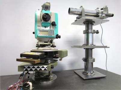
Fig. 2Equipment composition: 1 – PC, 2 – geodetic instrument, 3 – motor control unit, 4 – motor drive, 5 – angle encoder, 6 – autocollimator, 7 – autocollimator control unit, 8 – reflecting mirror, 9 – rotary table
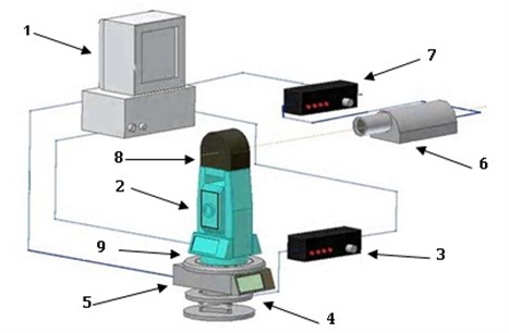
Fig. 3Main system structure, devices and connections
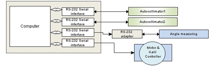
The block-diagram in Fig. 3 depicts the main system structure, devices used and the way that devices communicate with a computer. Each device is connected through RS-232 interface and operates as a regular COM port device. For angle measuring the Hewlett Packard’s HEDS-5310 high resolution incremental optical encoder is used. But because the voltage levels from it are not conforming to RS-232 standard, a small electronic circuit was made for correct functioning of the interface. The motor controller from GALIL has a true RS-232 interface and attached directly to a serial port on the computer.
The motor controller operates through the set of commands sent from computer. The command structure of the controller is organized as follows:
Nkppppppppppp < LF > or < CR >< LF >, (for example 4G2000 < LF >),
where:
n = address (ASCII 0...7 or 0...99 for customer specific base addresses),
k = command (ASCII Capitals and small letters as well as special characters),
p = parameter (ASCII decimal value with up to 10 digits plus negative sign, if applicable),
< CR > = carriage return 0DH; < LF > = line feed 0AH, whereas < CR > is ignored.
Each valid command with a valid address is followed by a feedback, which is structured as follows:
na < LF >, (e.g. 4* < LF>), where:
n = address (0...7) of the acknowledged module,
a = * or ! or #, which stand for:
– * = command accepted,
– # = erroneous parameter (exceeding the range),
– ! = command cannot be accepted (e.g. a new definition of the ramp or of a ramp range during a positioning process in ramp mode 1).
If there is no controller module with the corresponding address connected to the serial interface, or if the transmitted command is invalid, there will be no feedback.
Autocollimator 2 is used when performing a calibration of a multiangular prism (polygon). As mentioned in [8], the Hilger&Watts 12-sided (having 12 reflective surfaces) precision polygon is very frequently used for the tasks in the calibration laboratory of the Institute of Geodesy of Vilnius Gediminas Technical University (VGTU).
As was already stated in [8], both autocollimators were modified at Kaunas University of Technology by fitting the CCD matrices to the optical autocollimators and thus obtaining the digital output of measurements. Autocollimators return the position (in the horizontal axis) of the reflected mark (stroke) in the form of the number of pixels from the beginning of the axis.
3. Test system algorithms
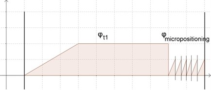
In order to perform various measurement instruments tests a number of methods should be used with corresponding functioning algorithm. These methods with some modifications are close to those described in [6]. The graph in Fig. 4 shows the main and most simple algorithm when the instrument under testing is moved to equidistant positions (10°, 30° etc.) by immutable ramp profiles.
The driving controller used in the system provides a range of ramp profiles that could be involved in different algorithms of system functioning. A trapezoid shaped ramp is used for implementing one of the algorithms described above (Fig. 5) [7]. The driving system accelerated constantly from 0 to the rated speed, then decelerates to a halt again when approaching the destination point.
If the set ramp is too flat in relation to the positioning distance, the rated speed will not be achieved. The deceleration process will then start exactly in the middle of the positioning distance, resulting in a triangular profile to be used (Fig. 6).
Fig. 4Speed and position dependency graph for equidistant positioning
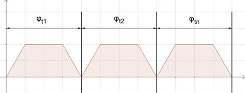
Fig. 5Trapezoid shaped ramp
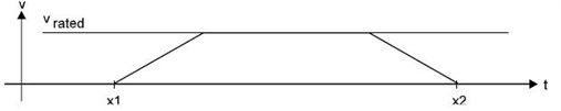
Fig. 6Triangular ramp
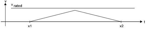
Such behavior is very useful while another positioning algorithm (Fig. 7) is used. Distances between points in micropositioning area are very close and thus the rated speed could not be achieved, that’s why triangular ramp profile helps to perform desired task.
Fig. 7Speed and position dependency graph for micropositioning
In order to achieve optimal and predictable results with regard to oscillation before coming to a predefined stop point, the driving controller offers 5 different configurable transmission functions or control parameters:
1. Proportional portion Kp,
2. Differential portion Kd,
3. Integral portion Ki,
4. Time constant for differential portion Td,
5. Pre-limitation of the integral portion Ri.
All these parameters could be adjusted by an appropriate command with some predefined range, wide enough to get high accuracy of speed control. For example, the range of proportional Kp gain is 0 – 255 and the optimal value is about 15.
4. Automatic control software design
The software implementing described earlier algorithms uses the well-known command design pattern described in [5]. Although the software implemented in .NET platform using C# programming language and the book explains the design patterns applied to Java language, all these patterns are common to all object oriented (OOP) programming languages.
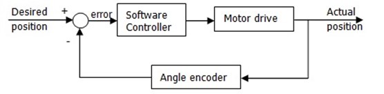
In the heart of command pattern lies the idea of “separating an object making a request from the objects that receive and execute those requests” [5]. That’s what we actually need because of the feedback line from the motor controller, which acts like a sensor in mechatronic system (Fig. 8). By such system design we could implement and use a number of commands, each of them taking responsibility of corresponding control logic, and execute this logic depending on the status message received from the control device through feedback line.
Fig. 8Automatic control system
The motor control unit sends the status feedback messages in the form of a character sequence or 8 byte word, like 10001001, each byte represents an individual bit holding deliberate information. In the meantime our automatic control software holds the table, or map of possible feedback messages sequences as keys, and corresponding objects of commands, implementing adequate logic, as map entries. An example of such a map is shown in Table 1.
Table 1Map of feedback messages
Key – status message | Object - Command |
10001101 | ZeroPositionReachedCommand |
00001000 | DriveStandsStillCommand |
00000000 | DriveRotatesCommand |
00001001 | PositionReachedCommand |
Each Command object implements Command interface with the sole method execute(), which implements the corresponding logic and is called right after the object is picked up from the map.
The diagram (Fig. 9) shows the interaction sequence between different system modules, depending on time and messages sent to each other.
Fig. 9System functioning sequence diagram
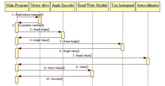
As could be seen from the diagram above, in the first place system obtains Zero position, the starting point of all measurements, stores its value and after this proceeds to other measurements.
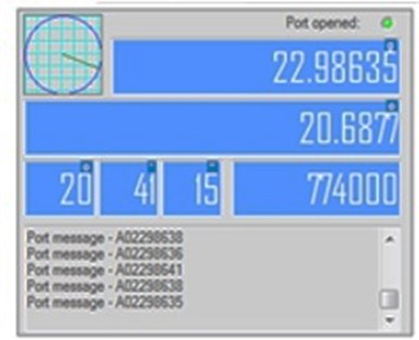
The user interface output of software (measurements bar) is shown in Fig. 10. The values are represented in gons, degrees, minutes, seconds and the remaining part of second. All values are stored in a local database for further processing.
Fig. 10UI output of software
5. Experimental results
In order to prove the concept described earlier in this paper, a set of experiments was performed in our Laboratory of Geodesy on the equipment represented and sketched in this paper. Generally, three attempts were taken, each of them consisting of 5 series of measurements on the full circle of 360 degrees taken from equidistant positions of 30 degrees. The total error was calculated by subtracting the value of a rotary table corrected by autocollimator value from the actual tachometer value:
The results of all three experiments are quite similar; therefore, the results of third experiment, having the least dispersion of values, are presented here. Fig. 11 depicts the results for total error.
Fig. 11Experiment No. 3 total error
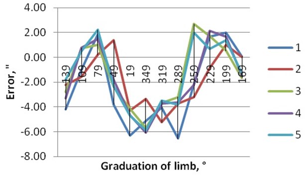
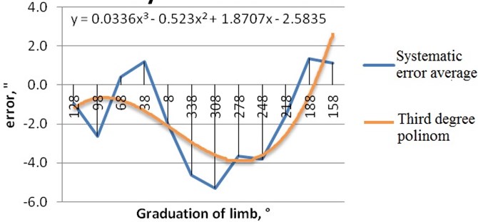
From the results of total error the systematic error emerges already. The figure (Fig. 12) shows the systematic error for all three experiments.
Fig. 12Experiment No. 1-3 systematic error
After we defined the systematic error, the error elimination algorithm could be chosen. From Fig. 13 it could be seen that systematic errors could be approximated by a third degree polynomial function.
Fig. 13Approximated polynomial function
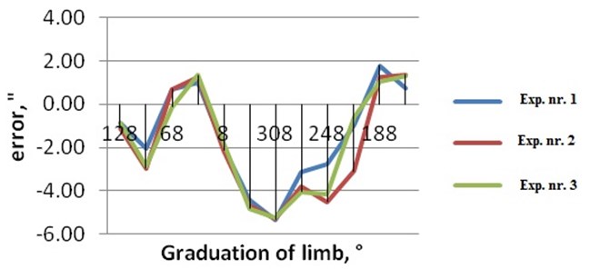
By eliminating systematic error according to the found algorithm the real tachometer error value is achieved. Fig. 14 shows this difference. The standard deviations before and after elimination of systematic error are shown in Table 2.
Fig. 14Experiment No. 3 tachometer error
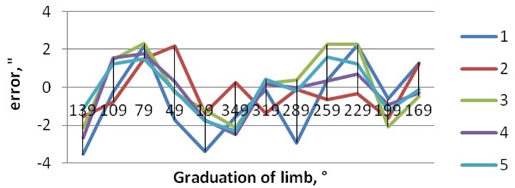
Table 2Standard deviations summary
Standard deviation | ||
No. | Total error, " | Systematic error eliminated, " |
1 | 1.54 | 0.89 |
2 | 1.65 | 0.80 |
3 | 1.69 | 0.90 |
Average | 1.63 | 0.86 |
Although the tachometer error after systematic error elimination remains high, it is reduced by half, as it could be seen from the standard deviation values.
6. Conclusions
A test bench for angle measuring geodetic instruments testing and calibrations was created and equipped by measuring software in Vilnius Gediminas Technical University, Institute of Geodesy. Created measuring information system allows performing the calibration of geodetic instruments with a sufficient precision. Nevertheless, further theoretical and practical research is needed to augment the accuracy of measurements.
References
-
Ingensand H. A new method of theodolite calibration. XIX International Congress of IMEKO, Helsinki, Finland, 1990, p. 91-100.
-
Bručas D., Giniotis V. The construction and accuracy analysis of the multireference equipment for calibration of angle measuring instruments. Proceedings of IMECO XIX World Congress: Fundamental and Applied Metrology, 2009, Lisbon, Portugal, Instituto Português da Qualidade, 2009, p. 1832-1837.
-
Katowski O., Salzmann W. The Angle Measurement System in the Wild Theomat T2000. Wild Heerbrugg Ltd., Precision Engineering, Optics, Electronics, Heerbrugg, Switzerland, 1983.
-
BIPM, IEC, IFCC, ISO, IUPAC, OIML. Guide to the Expressions of Uncertainty in Measurement. ISO Publishing, 1995.
-
Freeman E., Robson E., Bates B., Sierra K. Head First Design Patterns. O'Reilly Media, 2004.
-
Giniotis V., Grattan K. T. V. Optical method for the calibration of raster scales. Measurement, Vol. 32, Issue 1, 2002, p. 23-29.
-
IMG Drive Technology. User’s Manual MCS7000 Series. Ingenieurbüro M. Gysling Steuer- und Regeltechnik, Zürich.
-
Bručas D., Giniotis V., Augustinavičius G., Stepanovienė J. Calibration of the multiangular prism (polygon). Mechanika, Vol. 4(84), 2010, p. 635-641.
-
Probst R., Wittekopf R., Krause M., Dangschat H., Ernst A. The new PTB angle comparator. Measurement Science Technology, Vol. 9, 1998, p. 1059-1066.
About this article

This research is funded by the European Social Fund under the Project No. VP1-3.1-ŠMM-07-K-01-102.
