Optimization of cutting parameters using multi-objective evolutionary algorithm based on decomposition

2.1. Workpiece and tool materials

(1) The selected work material in this study is NAK80, the hardness of which is HB 344-400. Both the chemical composition and physical and mechanical properties are shown in Table 1 and Table 2 respectively.

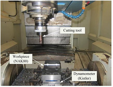
(2) The experimental study is carried out on a high-speed machining center VMC0745. Without any cutting fluid, the experiment is conducted in the style of down milling, as shown in Fig. 1. 9433 bench is used in the dynamometer, and cutting force acts on the Kilstler 9265B piezoelectric sensors to produce the charge signal, which can be amplified by multi-channel charge amplifier 5070. These signals are collected through data acquisition card and transmitted to the computer. The software of data processing (DynoWare) is used to test and analyze the collected signals. The surface roughness can be measured by MarSurf PS1, which is produced in Germany as a portable roughness measuring instrument.

Fig. 1Milling experiment

(3) The cutting tools are made of solid carbide and coated with TiSiN under major specifications, such as diameter of 16 mm ($\Phi$), teeth of 4, helix angle of 35, and the $R$ angle of 1.

2.2. Experimental design

The experiment is designed using the Taguchi method, which focuses on minimizing process variation or follows the least sensitive manner towards the environmental variation for products and process. The Taguchi method can also realize the robust and optimal operation under the varied environment conditions with high efficiency. Due to the material cutting principle, major influential factors are cutting speed ($v$), feed rate ($f$) and depth of cut ($d$). The width of cut ($w$) is fixed to 10 mm. The three factors are employed as cutting parameters to build experimental tables, and each factor is set three levels, shown in Table 3. The three factors with every three levels consist of L27 orthogonal array, shown in Table 4. The cutting force ($F$), surface roughness ($Ra$) and material removal rate ($MRR$) are engaged as responses.

3.1. Cutting force

Cutting force is one of the main physical phenomena in the metal-cutting process, which directly affects the cutting heat, tool wear, tool life and the quality of machined surface. Moreover, it can cause vibration, or even damage tools and machine parts. It is also essential in the design of machine tools, cutting tools and fixtures. Especially with the development of automated processing, cutting force is often used as a significant parameter in the adaptive control of cutting process and has been widely appreciated. Therefore, it is not only an important aspect of the cutting mechanism, but also significant for the application. Its statistical model based on regression method is developed by making use of the experimental results and given below:

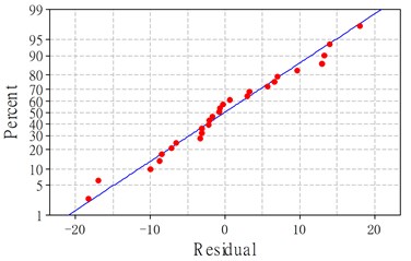
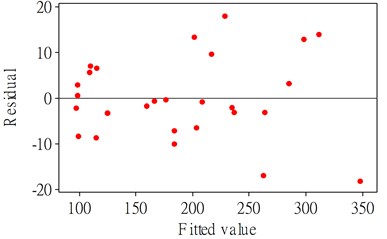
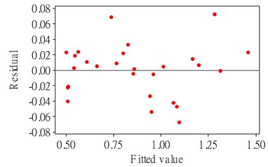
The $R^2$ value of the second-order polynomial model for cutting force is 97.8 %, it can be noted that this model is highly significant at a 95 % confidence level. It provides an excellent relationship between the response and the experimental values. A variance analysis of the model is shown in Table 5. It shows that all the cutting parameters and two-level interaction effect of cutting speed and depth of cut ($v\times d$), feed rate and depth of cut ($f\times d$) affect on the cutting force. The most significant factor associated with the cutting force is depth of cut, with 83.353 % contribution to the model. The residuals plot, including normal probability plot and residual versus fitted values for cutting force are presented in Fig. 2. It can be seen from Fig. 2a that the residuals fall on a straight line, which means that the errors between the experimental and predicted values are normally distributed, and the regression model is well fitted. Fig. 2b shows that the maximum variation is within the range from –20 to 20, which indicates the existence of high correlation between observed and fitted values.

Fig. 2Residuals plot for cutting force

a) Normal probability plot

b) Residual vs fitted values

3.2. Surface roughness

Surface roughness is one of the most important criteria for machining quality measurement. The performance and durability of mechanical parts are not only connected with the material and heat treatment, but also closely related to its surface micro-geometry or surface roughness. The surface roughness directly affects the wear resistance, corrosion resistance, fatigue strength and coordination properties of the mechanical parts:

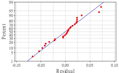
The model developed above establishes the relationship between the cutting parameters and the response of surface roughness in down milling of NAK80. Similarly to the cutting force, the $R^2$ value of second-order polynomial regression model for surface roughness is over 98 %, which means that the statistical model reflects the relationship between the cutting parameters and the response. The analysis of variance table of the statistical model for $Ra$ is presented in Table 6, which indicates that the model is highly significant at a 95 % confidence level for that the probability is less than 0.05. Fig. 3a displays the normal probability of residuals for $Ra$, which indicates that the model is well suited for the residuals that are distributed normally and falls in a straight line. The fitted value versus the residuals are shown in Fig. 3b, which shows a high correlation that exists among the experimental values, the model for the residuals is within the range from –0.08 to 0.08 as can be observed.

The comparison between the predicted and measured values for cutting force and surface roughness is shown in Fig. 4. Through the analysis and comparison, it indicates that the two statistical models both have a high accuracy and can be used for the optimization instead of the actual model.

Fig. 3Residuals plot for surface roughness

a) Normal probability plot

b) Residual vs fitted values

Fig. 4Comparison between predicted and measured values

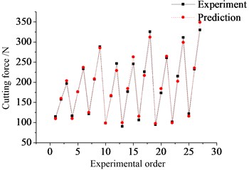
a) Cutting force

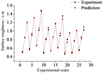
b) Surface roughness

4.1. Cutting force

Table 5 shows that cutting speed ($v$), feed rate ($f$), depth of cut ($d$), two-level interaction effect of cutting speed and depth of cut ($v\times d$), feed rate and depth of cut ($f\times d$) all have significant effect on the cutting force. In Fig. 5a it can be seen that the lowest cutting force can be attained with the combination of the highest cutting speed and smallest depth of cut. The effect of feed rate and depth of cut on cutting force is depicted in Fig. 5b. In the two figures it can be found that along a fixed depth of cut, the cutting force does not change obviously with the increase of cutting speed or feed rate. In other words, the influence of depth of cut is the largest, which can also be determined from the analysis of variance above (Cont. ≈ 83.353 %). The other two critical factors are cutting speed and feed rate with contributions 2.02 % and 7.776 % respectively. Among two-level interaction effects, only the interaction of cutting speed and feed rate has a very weak significance with 0.003 % contribution. The variation of cutting force with each of the cutting parameters in a given range is shown in Fig. 5c, which indicates that the cutting force is growing with the increase of each single factor, but has only a small change for cutting speed.

Fig. 5Effect of cutting parameters on cutting force

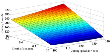
a) Interaction effect of cutting speed and depth of cut ($f=$ 0.56 mm·rev^-1)

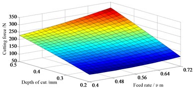
b) Interaction effect of feed rate and depth of cut ($v=$ 120 m·min^-1)

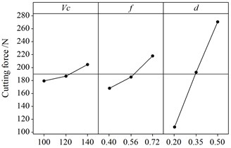
c) Main effect of cutting parameters

4.2. Surface roughness

Concerning surface roughness, the analysis of variance is summed up in Table 6. Fig. 6a shows the experimental response surface for $Ra$ in relation to cutting speed and depth of cut, while the feed rate is kept at the middle level. The lowest surface roughness is achieved at the highest cutting speed and smallest depth of cut. And it is depicted that the higher the cutting speed or the smaller the depth of cut, the lower the surface roughness will be. This regular pattern can also be found from Fig. 6b. Like cutting force, the factor ($d$) affects surface roughness in a considerable way and the contribution of three cutting parameters is over 93 %. However, the effect of feed rate on the surface roughness is larger than cutting speed while the situation is different on the cutting force. Besides the interaction of cutting speed and depth of cut ($v\times d$), other factors do not present any statistical significance on the surface roughness.

Fig. 6Effect of cutting parameters on surface roughness

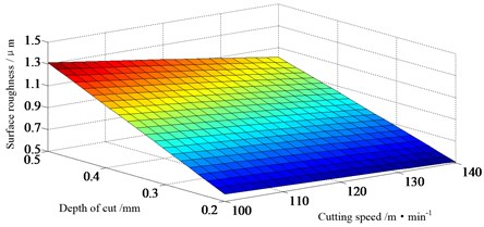
a) Interaction effect of cutting speed and depth of cut ($f=$ 0.56 mm·rev^-1)

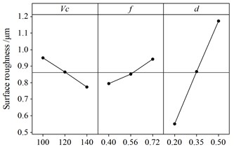
b) Main effect of cutting parameters

5.1. Multi-objective evolutionary algorithm based on decomposition

A multi-objective optimization problem for engineering application and scientific research can be expressed as:

where $\Omega$ dominates the feasible region of parameters, and $F:\Omega \to R^m$ consists of $m$ real-valued functions with the space of objective function $R^m$.

The method of MOEA/D was introduced by Zhang in 2007 [15], combining the traditional mathematical programming with the evolutionary algorithm. In his paper, the MOP is decomposed into $N$ single objective scalar optimization sub-problems, and each sub-problem is solved by evolutionary algorithm. The population of the evolutionary algorithm is generated from the current optimal solutions of each optimization sub-problem. Then the neighborhood of each pairwise sub-problem is defined as the distance of the couple weights, and the optimization of each sub-problem can be solved by means of evolving manner among the neighbor sub-problems.

Let ${\lambda }^1,\cdots ,{\lambda }^N$ be a group of weight vectors distributing uniformly, $z^{*}$ as the reference point. Through the Tchebycheff method, the MOP problem can be decomposed into $N$ scalar optimization problems, in which the objective function of the $j$-th sub-problem is:

where ${\lambda }^j={({\lambda }_1^j,{\lambda }_2^j,\cdots ,{\lambda }_m^j)}^T$ and $g^{te}$ is continuous with respect to $\lambda$. The optimal solution of $g^{te}\left(x\right|{\lambda }^i,z^{*})$ should be close to that of $g^{te}\left(x\right|{\lambda }^j,z^{*})$ while ${\lambda }^i$ is close to ${\lambda }^j$. It means that any information close to ${\lambda }^i$ about $g^{te}$ will contribute to $g^{te}\left(x\right|{\lambda }^i,z^{*})$.

In MOEA/D, the neighbor of weight vector ${\lambda }^i$ is defined as the nearest neighbors of its surround weight vectors $\{{\lambda }^1,\cdots ,{\lambda }^N\}$. Therefore, the neighbor of the $i$ sub-problem consists of sub-problems which are the nearest neighbor weight vectors to ${\lambda }^i$. The optimization of each sub-problem could only be solved by its own surrounding neighbors. In every evolved generation, MOEA/D has the following parameters: 1) the population with size $N:x_1,\cdots ,x_N\in \Omega$, where $x_i$ is the current solution of the $i$-th sub-problem, 2) $z={(z_1,\cdots ,z_m)}^T$, where $z_i$ is the best value of $f_i$, 3) archive set $A$ is used to store the non-dominated solutions during the optimal process. Stated procedurally, the step of MOEA/D is as follows.

(1) Initialization

• Set the number of evolution iterations as $t^{\mathrm{m}\mathrm{a}\mathrm{x}}$, the number of sub-problems as $N$, weight vectors as ${\lambda }^1,\cdots ,{\lambda }^N$, and the number of neighbor weight vectors for each vector as $T$.

• Let $A=\varphi$. Calculate the distance between every two weight vectors and get the $T$ neighbor weight vectors for ${\lambda }^i$.

• Let $B\left(i\right)=\{i_1,\cdots ,i_T\}$ ($i=1,\cdots ,N$), where ${\lambda }^{i_1},\cdots ,{\lambda }^{i_T}$ are the neighbor weight vectors for ${\lambda }^i$.

• Initialize the population $x_1,\cdots ,x_N\in \Omega$ randomly, calculate $F\left(x_i\right)$ and then initialize $z={(z_1,\cdots ,z_m)}^T$.

(2) Iterative calculation

Run the following operations for $i=1,\cdots ,N$:

• Recombination: individuals $x_k$ and $x_i$ are randomly selected from $B\left(i\right)$ and then recombined to form a new individual $y$.

• Mutation: $y$ is randomly mutated to form $y^{\text{'}}$.

• Update $z:z_j=f_j\left(y^{\text{'}}\right)$ if $z_j<f_j\left(y^{\text{'}}\right)$ ($j=1,\cdots ,m$).

• Update the neighbor individuals: $x^j=y^{\text{'}}$ and $F\left(x^j\right)=F\left(y^{\text{'}}\right)$ if $g^{te}\left(y^{\text{'}}\right|{\lambda }^j,z)\le g^{te}(x^j|{\lambda }^j,z)$, where $j\in B\left(i\right)$.

• Update archive set $A:$ delete the vectors in $A$ dominated by $F\left(y^{\text{'}}\right)$, and then add $F\left(y^{\text{'}}\right)$ to $A$.

• Termination condition

If the termination condition is satisfied, output the archive set $A$. Otherwise, back to (2).

5.2. Results and discussion

Based on the above algorithm, MOEA/D is performed to optimize the cutting parameters for the purpose of convergence to the real Pareto boundary. The solutions should have diversity and uniformity and cover the entire boundaries as possible. There is not only a global optimal solution existing in the multi-objective optimization, but also solution sets. The objective functions, derived from equations (2) and (3) and the theoretical formula (1) of material removal rate, can be expressed as follows:

The initialized parameters of MOEA/D are: evolution generations 1000, population size 100, neighbor numbers 20 and decomposition method of Tchebycheff. The final solution sets, composing the Pareto front shown in Fig. 7, are obtained over the entire optimization and 10 out of them are presented in Table 7. Here any solution in the final set is not persuasively better than others, for each one of them can be regarded as the optimal solution under the specific product requirement. Therefore the process engineer should select the optimal solution reasonably. A suitable combination of cutting parameters can be selected from Table 7 if the engineer desires to have a smaller cutting force, a better surface finish or a higher material removal rate.

Fig. 7Pareto optimal front using MOEA/D for three objectives

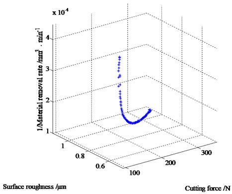
From the experimental results presented in Table 4, the responses of order 1 obtained are as follows: $F$ (114.6 N), $Ra$ (0.523 μm) and $MRR$ (1591.55 mm³/min). After optimization of cutting parameters using MOEA/D, it can be seen that $F$ and $Ra$ has been respectively reduced to 109.12 N and 0.5 μm for the approximately same material removal rate (order Table 7).

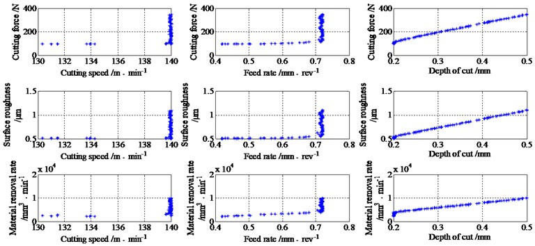
The varied results obtained from MOEA/D for the responses of cutting force, surface roughness and material removal rate with respect to different cutting parameters are presented in Fig. 8. According to the figure, it can be asserted that most of the Pareto optimal points are concentrated on higher cutting speed, higher feed rate and at a lower depth of cut. Therefore, it can be used as the basis to combine the cutting parameters by engineers.

Fig. 8Pareto optimal solutions with respect to individual cutting parameters