Detection of low-dimensional chaos in drill bit torsional vibration time series

2.1. The installation of the measurement system

The present MWD surveying system incorporate three-axis magnetometers and three-axis accelerometers arranged in three mutually orthogonal directions [15, 16], which are installed inside the nonmagnetic drill collar. This special drill collar is usually designed for Monel metal to avoid the external interferences with the measurements taken by the magnetometers [17]. Aboelmagd Noureldin [18] proposed that the nonmagnetic drill collar too expensive and developed the technology of fiber optic gyroscopes (FOG) has been suggested for MWD surveying of directional wells [19]. But gyroscope’s reliability is a problem, so this paper focuses on the magnetic surveying tools that have a wider range of applications. The installing structure of the downhole measurement system shows in Fig. 1. That is conducted by triaxial accelerometer and triaxial magnetometers, and redundancy design is adopted.

Fig. 1Measurement system (Left is the simplified diagram of bottom-hole assembly; Middle is the construction of measurement system; Right is installed structure of sensors)

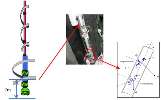
Assume the acceleration of gravity as $G$, Earth’s magnetic field strength as $F$. $g_x$, $g_y$, $g_z$ are respectively defined as survey gravity signals of triaxial accelerometers on the $xyz$ axis, obviously, $G=\sqrt{g_x^2+g_y^2+g_z^2}\text{.}$$f_x\text{,}$$f_y\text{,}$$f_z$ are respectively defined as survey signals of triaxial magnetometers on the $xyz$ axis, and $F=\sqrt{f_x^2+f_y^2+f_z^2}$. When the rotational speed of the drillstring is 120 r/min, it can generate 50 measurement velocity data points when the drillstring rotates one lap.

Performance characteristics of the accelerometers and magnetometers are summarized in Table 1.

2.2. Calculation of the drill bit rotational speed

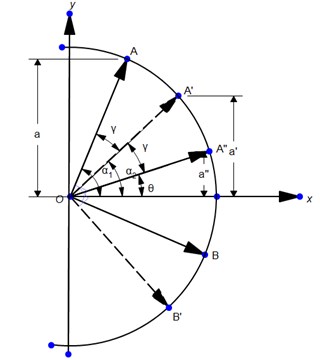
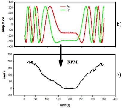
In the process of drilling, a magnetometers in the center of the drillstring will draw an approximate sinusoidal course with the drillstring rotation, but the drillstring rotation speed is variable, so the measurement curve is not strictly sinusoidal (Fig. 2(b)). From the theoretic point of view, a single axis magnetometer signal should be sufficient for the determination of the drillstring rotational speed, as shown in Fig. 2(a). Assuming that the drill callor radius is $r$, $OA$ is a central axis direction of the magnetometer, $F_h$ is the horizontal projection of the Earth’s magnetic field, obviously, $r\propto F_h$, after the time $\mathrm{\Delta }t$, $2\mathrm{\Delta }t$, respectively, magnetometer rotates to $OA\text{'}$, $OA\text{'}\text{'}$ from $OA$, when the measured values are proportional to $a$, $a\text{'}$, $a\text{'}\text{'}$. The following equtions can be obtained:

where $f_{x,y}$ expressed $f_x$ or $f_y$ which any one, we can solve the angle $\gamma$ according the Eq. (1)-(3):

The drillstring rotates the angle of $\gamma$ in the time of $\mathrm{\Delta }t$, accordingly solving the rotation speed. This equation, however, is the inverse cosine function, whose definition domain is $\left|(a/a\mathrm{\text{'}}\mathrm{\text{'}}+1)/(2\cdot a\mathrm{\text{'}}/a\mathrm{\text{'}}\mathrm{\text{'}})\right|\le 1\text{.}$ This characteristic will bring a challenge in downhole data processing.

Because $\gamma ={\alpha }_1-{\alpha }_2$ and the triaxial magnetometers were mounted vertically with each other on the $xyz$ axis, there will be 90° phase difference between $f_x$ and $f_{\mathrm{y}}$, as shown in the Fig. 2(a). When $f_x$ transfers from $OA$ to $OA\text{'}$, $f_y$ will transfer from $OB$ to $OB\text{'}$ at the same time. The measurement signals as show in Fig. 2(b) is obtained from filed experiments.

Then:

Fig. 2The fluxgate rotation measurement calculation of the rotation speed diagram

a)

Thus ${\alpha }_1=\mathrm{a}\mathrm{r}\mathrm{c}\mathrm{t}\mathrm{a}\mathrm{n}\left(f_x/f_y\right)$, drillstring rotational speed ($RPM$) can be defined as follows:

The definition domain of arctangent is $(-\mathrm{\infty },+\mathrm{\infty })$, superior to the former algorithms. The speed value calculated is determined using the moving average filter for further processing, according Eq. (7). The smooth results as show in Fig. 3, therefore, it is conducive for the subsequent analysis when the speed value is smoother:

Fig. 3Rotational speed time series (using 10000 data points)

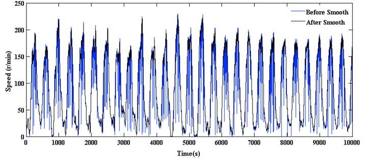
Finally, the drillstring $RPM$ time series is shown in Fig. 2(c) and Fig. 3. Since using synchronization calculating, it can be considered that the sampling rate of the rotational speed is 100 Hz. The dynamics of the drill bit torsional vibration will be revealed by the following nonlinear analysis of the measurement signal time series.

Assume the drill bit rotational speed time series finally resolved as ${\omega }_0$, ${\omega }_1$,…, ${\omega }_n$, then the time series of rotation angle is ${\theta }_0$, ${\theta }_1$,…, ${\theta }_n$, sampling frequency is $f=1/\mathrm{\Delta }t=$100 Hz, then the rotation angle and rotation speed satisfy the following equation:

3.1. Phase-space reconstruction

The dynamics of the time series $x_0$, $x_1$,…, $x_{n-1}$ are fully captured or embedded in the $m$-dimensional phase space, $m\ge d$ where $d$ is the dimension of the original attractor. A vector ${\overrightarrow{x}}_i$ in the reconstructed phase space is constructed from the time series as follows:

where $\tau$ is the delay time.

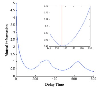
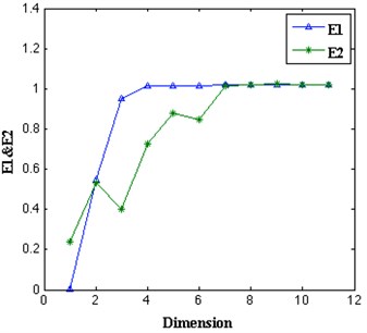
We apply the mutual information [20] to estimate a proper embedding delay $\tau$, Fraser and Swinney [20] considered to use the first minimum of the mutual information as the optimal embedding delay. The first minimum of the mutual information calculated for the rotational speed time series is obtained at $\tau =$157 (Fig. 4(a)), which is also the value that we will use in all-subsequent calculations. We use Cao’s method [21] to determine the embedding dimension. It computes $E_1$ and $E_2$ for the data set of dimension 1 up to a dimension of $D$ which is the largest embedding dimension used for calculating. $E_1$ and $E_2$ are defined as follows:

wherein $d$ is the embedding dimension, $N$ is the number of data points, $\tau$ is the embedding delay, $x_{i+d\tau }$ and $x_{n(i,d)+d\tau }$ is the $i$th vector in the data sets and its nearest neighbors of $d$-dimensional phase space [22]. Calculating both $E_1\left(d\right)$ and $E_2\left(d\right)$ to determine the minimum embedding dimension of the time series, and to distinguish deterministic data from random data. As shown in Fig. 4(b), clearly the minimum embedding dimension is 7.

The signals, which have chaotic characteristic, usually seem to be random, especially when the nonlinear invariants are similar to the noise. We are not fully aware of the nature of the drillstring vibration signals that perform as time series, the fluctuation of parameter $E_2$ in the Cao’s method can be used as a measurement of uncertainty. When the system is chaos, $E_2$ will gradually increase to one from zero as the embedding dimension increases. When the random of the sequences enhances, the fluctuation range of $E_2$ will become smaller and smaller, finally, $E_2$ will approach to constant when the system is completely random, since there is no correlation between the data sets.

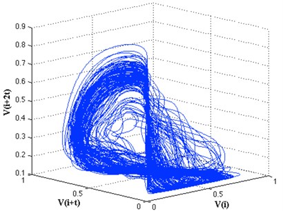
Having calculated the optimal $\tau$ and $m$, we are able to successfully reconstruct the phase space of the system. For $\tau =$ 157 and $m=$ 7, the 3D projection of the attractor obtained according to Eq. (9) is presented in Fig. 5. The correct phase space reconstruction is a key step that enables further analysis of the dynamics associated with the torsional vibration.

Fig. 4Determination of the proper delay time and embedding dimension of the torsional vibration: a) the mutual information has the first minimum at τ= 157, b) the minimum embedding dimension is 7

a)

b)

Fig. 5Three-dimensional projection of the reconstructed phase space (obtained with embedding parameters: τ= 157 and m= 7)

3.2. Stationarity test

Since linear statistics, such as the mean or standard data deviation, usually do not possess enough discrimination power when analyzing irregular signals, nonlinear statistics have to be applied. We apply the stationarity test [23] program “stationarity.exe” [24] provided by [24] Matjaž Perc. They split the time series into several short non-overlapping segments and then use a particular data segment to make predictions in another data segment. By calculating the cross-prediction error (${\delta }_{gh}$) when considering points in segment $\mathrm{g}$ to make predictions in segment $h$, the cross-prediction error as a function of $g$ and $h$ then revels which segments differ in their dynamics. They obtained a very sensitive statistic capable of detecting changes in dynamics and thus a very powerful probe for stationarity.

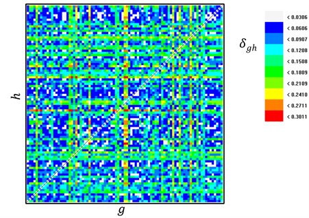
The average cross-prediction errors for all possible combinations of $g$ and $h$ are presented in Fig. 6. The whole time series was partitioned into 56 non-overlapping segments each occupying 1000 data points. The average value of all ${\delta }_{gh}$ is 0.17, while the minimum and maximum values are 0.03 and 0.3, respectively. Since the maximal cross-prediction error is not one time larger than the average, we can determine that the studied time series is stationarity. We just consider only 1000 s of the torsional vibration time series. Otherwise, longer data sets of the vibration time series almost yield non-stationary.

Fig. 6Stationarity test. The color map displays average cross-prediction errors δgh in dependence on different segment combinations

3.3. Correlation dimension

After the reconstruction of time series in phase space, we can determine whether it have chaotic properties by calculating the chaotic invariants. Common chaotic invariants are correlation dimension [14], Kolmogorov entropy [25] and the Lyapunov exponent [26] and so on. The correlation dimension method is used for detecting the presence possibility of chaos. An algorithm proposed by Grassberger and Procaccia [14] is the most commonly applied method. According to this method the correlation sum, $C\left(r\right)$, is expressed as:

where $H$ is Heaviside step function defined as:

$N$ is the number of points in time series; $r$ is the radius of a sphere with its center at either of current points.

Then the correlation dimension is:

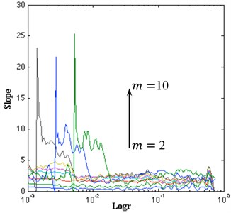
For the random process, $D_2$ varies linearly with increasing without reaching a saturation value. If the system is chaotic, the slope of $\mathrm{l}\mathrm{o}\mathrm{g}C\left(r\right)$ vs $\mathrm{l}\mathrm{o}\mathrm{g}r$ converges to $D_2$ over an appropriate interval as $m$ increase.

In Fig. 9(a) we present the estimated slope as a function of $\mathrm{l}\mathrm{o}\mathrm{g}r$ for embedding dimensions $m=$ 2 up to 10, where we see that a possible region of convergence the scaling region $\mathrm{l}\mathrm{o}\mathrm{g}r$ in the interval [–1.8, –0.6]. The estimated correlation dimension along with the estimated error as a function of the embedding dimension is presented in Fig. 9(b). We can estimate a correlation dimension in the range 2.0-3.0. This behavior indicates the possible existence of low-dimensional attractor with an estimated as $D_2=\text{2.4±0.2}$.

Fig. 9a) Local slope of correlation sum; b) estimated dimension of the attractor for the data set

a)

b)

3.4. Largest Lyapunov exponent (LLE)

The basic characteristics of chaotic motion are that the movement is extremely sensitive to initial conditions, two very close initial values resulting in orbit over time by separating exponentially, Lyapunov exponent [26-28] that describes the amount of this phenomenon.

Suppose chaotic time series is $\left\{x_1,x_2,\dots ,x_n\right\}$, embedding dimension is $m$, time delay is $\tau$, then reconstruction phase space is:

Take the initial point of phase space as $Y\left(t_0\right)$, suppose that its most neighboring point is $Y_0\left(t_0\right)$, the distance between two points is $L\left(t_0\right)$, from time $t_0$ to start tracking the time evolution of these two points, until the space between the two points exceeds a predetermined value $\epsilon$ on the moment $t_1$:

Retain point $Y\left(t_1\right)$, suppose its most neighboring point as $Y_1\left(t_1\right)$, then:

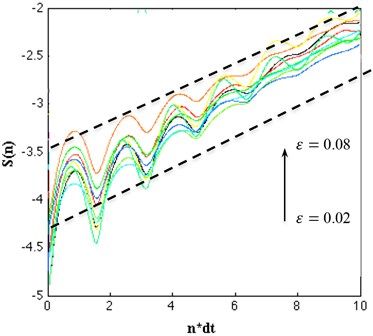
Fig. 10Calculation of the maximal Lyapunov exponent of the torsional vibration, the effective expansion rate S(n), of which the linear slope in dependence on n*dt (dt= 0.01) is a robust estimate for the largest Lyapunov exponent

And makes the angle $\theta$ between $L\left(t_1\right)$ and $L\text{'}\left(t_1\right)$ as small as possible, repeat the above procedure until $Y\left(t\right)$ reaches the end of the time series, the total number of iterations is $M$, then the Largest Lyapunov exponent will be obtained:

In order to estimate the largest Lyapunov exponent we employed the methodology of Kantz [26] using the program “lyapmaxk.exe” [27] provided by Matjaž Perc. The results obtained for $\epsilon =\text{0.02-0.08}$ are presented in Fig. 10. The function $S\left(n\right)$ shows a rather robust linear increase from $n=$500 to 1000 for all $\epsilon$. Thus, the slope of $S\left(n\right)$, indicated by the two linear lines, is a good estimate for the largest Lyapunov exponent of the system. The largest Lyapunov exponent is calculated through least-squares line fit for the time series and is found to be 0.15. This positive value indicates exponential divergence of trajectories and hences an evidence of chaos.