A new crack diagnosis method on box structure based on empirical mode decomposition

1. Introduction

Most spacecrafts are valuable, unique and unrepairable on orbit, so high reliability is a basic requirement for spacecrafts. So it is an important subject how to diagnose the damage of the spacecraft structure.

Dynamics environmental testing is an essential part in the process of developing spacecrafts. In the current process of spacecrafts development, feature-level structure response curves are referred to diagnose the damage of the structure. In detail, the estimation of the existence of frequency excursion or amplification of the response data before and after the high-level or random vibration test is performed. It is just a kind of qualitative analysis, and the form, the location and other information of the damage cannot be deduced. These necessary features rely on human’s judgment, and sometimes the check inside the structure is required, which is very time consuming [1].

Empirical mode decomposition is a rising kind of signal processing method in recent years, which is suitable for non-linear and non-stationary signals. This method is applied here to process the vibration signals of a two-level box in order to diagnose the crack of the box, as a primary exploratory study for application to the field of spacecraft structural fault diagnosis.

2. Empirical mode decomposition

Empirical Mode Decomposition (EMD) is an important part of the Hilbert-Huang transform, by which a time-domain signal is decomposed into a collection of intrinsic mode functions. An intrinsic mode function (IMF) satisfies two basic conditions: (1) in the whole time range, the number of extrema and the number of zero crossings must either equal or differ at most by one; and (2) at any point, the mean value of the envelop defined by the local maxima and the envelop defined by the local minima is zero. An IMF is not restricted to a narrow band signal, and it can be both amplitude and frequency modulated.

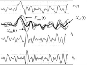
Having defined IMF, the original vibration signal should be divided into a series of IMFs. This process is known as the decomposition. After integrating all components, final results can be obtained. A schematic of the process to identify intrinsic mode functions of a signal is shown in Fig. 1.

The mean of the upper and lower extrema curves is defined as:

Fig. 1The process of obtaining intrinsic mode functions

Subtracting the mean from the original signal, the first estimate of an intrinsic mode function is obtained:

This process is called filtering which result in the third curve shown in Fig. 1. But $h_1$ usually does not satisfy the conditions of an IMF, and further filtering is usually needed. The next filtering assumes that $h_1$ is the signal and the mean from $h_1$ is $X_{m_{11}}\left(t\right)$, so that the next estimate becomes:

After $k$ filtering, we define the first IMF to be:

To obtain the second and subsequent IMF, the residual signal can be computed as:

The residual, $r_1\left(t\right)$, now becomes the new data that can be subjected to the same filterting process to extract more IMFs. This process is repeated to obtain $c_2\left(t\right)$ through $c_n\left(t\right)$ IMFs. By summing up all of the IMFs, it is possible to represent a vibration signal as:

Thus, the original data $X\left(t\right)$ has been divided into $n$ empirical modes, $c_n\left(t\right)$ and a residue $r_n\left(t\right)$ [2, 3].

In this paper, EMD method is used to track the damage in a two-story box, by the time-domain vibration response signals of the structure, in order to obtain more information about the crack in the board.

3. The FEA of a box structure

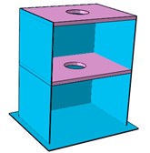
Box structures are widely used, such as the main structure of small satellites, or the sub-structure of large spacecrafts. So a box structure is selected here. The schematic diagram of a two-story box is shown in Fig. 2(a). Bottom/side boards are Al5052 and top/clap boards are Aluminum honeycomb sandwich structures.

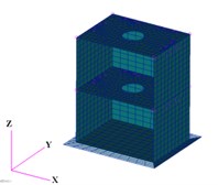
This box structure is modeled in MSC.Patran2011 and analyzed in MSC.Nastran2011.1. The finite element model of the box is illustrated in Fig. 2(b). Two different cases are assumed, with an undamaged box in case 01 and a $y$-direction crack in the top board of the box in case 02.

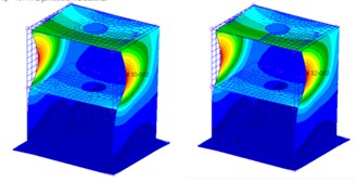
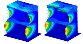
The model is bottom fixed, whose first four modes are calculated. The natural frequencies are shown in Table 1, and the mode comparison is presented in Fig. 3.

Fig. 2A two-story box model

a)

b)

Fig. 3The mode comparison of two cases: a) first-order mode: case 01 is left and case 02 is right; b) fourth-order mode: case 01 is left and case 02 is right

a)

b)

According to all above analysis, the difference about natural frequencies and modes between two cases is slight so it is hard to tell the fault of the structure. Thus, a new method is needed to diagnose the failure of a structure.

4. Testing and analysis

4.1. The vibration test

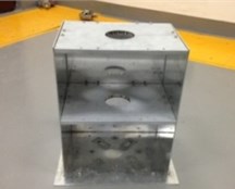
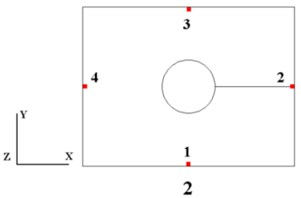
The real two-story box is shown in Fig. 4, whose parameters are the same as the FEM model.

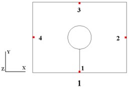
Fig. 4The box structure and a schematic diagram of board 1

a)

b)

Two cases have been assumed as above. A board with a y-direction crack is designed to simulate case 02 shown in Fig. 4(b). The coordinate is the same as that in Fig. 2(b). Sine sweep vibration is adopted, whose sweep rate is 4 oct/min, frequency range from 5 to 500 Hz and testing level is 0.1 g. The sensors are set in the middle of four edges of the top board, illustrated in Fig. 4(b), which measure three axial acceleration responses.

4.2. Analysis

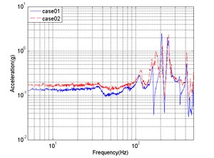
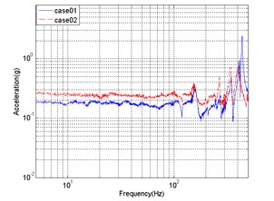
After vibration tests, the acceleration response data are obtained. Based on the frequency response data, the curve of case 02 is similar to that of case 01, shown in Fig. 5.

Fig. 5The contrast between two cases’ frequency response: a) x-direction input, sensor 1 x-direction response; b) y-direction input, sensor 4 y-direction response

a)

b)

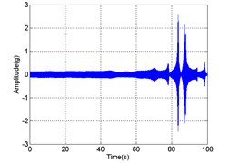
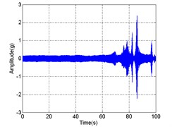
Fig. 6Time-domain curves, x-direction input, sensor 1 x-direction response; a) case 01 and b) case 02

a)

b)

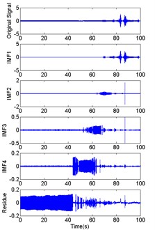
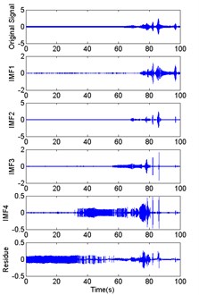
Fig. 7EMD processes, x-direction input, sensor 1 x-direction response; a) case 01 and b) case 02

a)

b)

Due to boundary effect, energy leakage and some other causes, higher IMFs always have no physical meanings. In fact, not so many filtertings are needed for analyzing. In order to ensure the accuracy and decrease the computation, here former four order IMFs are decomposed, and higher than fourth-order IMFs are considered to be residue.

The time-domain data from the same sensor in different cases share some resemblance, as shown in Fig. 6. The EMD processes to time-domain data are illustrated in Fig. 7.

The vibration signal can be devided into $n$ IMFs, $c_1\left(t\right)\text{,}{c}_2\left(t\right)\text{,…,}{c}_n\left(t\right)$, and a residue $r_n\left(t\right)$, then the energy of each IMFs, $E_i$, and the energy of residue, $E_r$, can be obtained by:

7

$E_i={\int }_{-\infty }^{+\infty }{\left|c_i\right(t\left)\right|}^{2}dt,E_r={\int }_{-\infty }^{+\infty }{\left|r_n\right(t\left)\right|}^{2}dt.$

A tag vector $\mathbf{T}$ is defined by all $E_i$, and $E_r$ as:

8

$\mathbf{T}=\left[E_1,E_2,\dots ,E_n,E_r\right].$

As the amount of energy is always large, define total energy $E=\sqrt{\left(\sum _{i=1}^n{\left|E_i\right|}^2\right)+{\left|E_r\right|}^2}$ and energy percentage, $R_i=E_i/E$ and $R_r=E_r/E$, then $\mathbf{T}$ is normalized as:

9

$\mathbf{t}=\left[R_1,R_2,\dots ,R_n,R_r\right].$

Assuming that the tag vector of the undamaged structure is ${\mathbf{t}}_0$ and that of the damaged is $\mathbf{t}$, in order to measure the angular separation of two vectors, a tag angle $\alpha$ is defined as:

10

$\alpha ={\mathrm{c}\mathrm{o}\mathrm{s}}^{-1}({\mathbf{t}}_0\cdot \mathbf{t}).$

So the information of the damage can be deduced from the tag angle $\alpha$.

Table 2The analyzed results of case 01 and case 02

Case number	Input/Output direction	Sensor number	Tag vector $\mathbf{t}$	Tag angle $\alpha$ (rad)
01	$x/x$	1	[0.995 0.071 0.018 0.021 0.070]	–
		2	[0.978 0.087 0.030 0.024 0.183]	–
		3	[0.672 0.226 0.146 0.127 0.679]	–
		4	[0.980 0.035 0.064 0.030 0.184]	–
	$y/y$	1	[0.989 0.026 0.028 0.021 0.144]	–
		2	[0.986 0.089 0.048 0.026 0.130]	–
		3	[0.985 0.084 0.045 0.025 0.138]	–
		4	[0.983 0.099 0.057 0.022 0.140]	–
	$z/z$	1	[0.999 0.015 0.006 0.003 0.004]	–
		2	[0.610 0.102 0.104 0.137 0.767]	–
		3	[0.570 0.122 0.103 0.148 0.792]	–
		4	[0.558 0.133 0.128 0.158 0.793]	–
02	$x/x$	1	[0.429 0.862 0.236 0.089 0.101]	1.046
		2	[0.535 0.793 0.139 0.097 0.237]	0.873
		3	[0.331 0.658 0.128 0.130 0.651]	0.559
		4	[0.598 0.717 0.168 0.099 0.299]	0.823
	$y/y$	1	[0.983 0.117 0.062 0.042 0.123]	0.102
		2	[0.861 0.405 0.189 0.102 0.221]	0.388
		3	[0.972 0.178 0.094 0.033 0.120]	0.109
		4	[0.859 0.409 0.208 0.063 0.219]	0.379
	$z/z$	1	[0.999 0.014 0.008 0.002 0.008]	0.005
		2	[0.421 0.310 0.133 0.164 0.826]	0.291
		3	[0.225 0.358 0.175 0.173 0.872]	0.437
		4	[0.327 0.293 0.171 0.166 0.867]	0.294

The sine vibration response signals are decomposed and analyzed as above, the results obtained shown in Table 2.

The crack is along the $y$ direction, orthogonal to the $x$ direction in case 02, which is close to sensor 1. According to Table 2, when loading $x$-direction input, the tag angle of sensor 1 is larger than that of any other sensor. But when loading other direction input, the feature of tag angle cannot be distinguished.

4.3. Verification

In order to verify the effectiveness of the damaged feature extraction, a board with an $x$-direction crack is designed to simulate case 03 illustrated in Fig. 8. Testing conditions are the same as above.

Fig. 8A board with an x-direction crack: board 2

The vibration response signals of case 03 are decomposed and analyzed as above, the results obtained partially shown in Table 3.

In case 03, the crack is along the $x$ direction, orthogonal to the $y$ direction, which is close to sensor 2. Similarly, based on calculation, when loading $y$-direction input, the tag angle of sensor 2 is larger than that of any other sensor, as shown in Table 3. But when loading other direction input, the feature of tag angle cannot be distinguished. So the effectiveness of the damaged feature extraction can be verified. To sum up, combined with the loaded input direction, the position and direction of a crack can be deduced on the basis of tag angle $\alpha$.

Table 3Part analyzed results of case 03

Case number	Input/Output direction	Sensor number	Tag vector $\mathbf{t}$	Tag angle $\alpha$ (rad)
03	$y/y$	1	[0.966 0.053 0.120 0.052 0.218]	0.127
		2	[0.906 0.378 0.102 0.037 0.155]	0.307
		3	[0.955 0.256 0.083 0.042 0.116]	0.182
		4	[0.945 0.291 0.083 0.037 0.119]	0.199

5. Conclusion

In this paper a two-story box structural response signals are empirical mode decomposed. According to IMFs, tag vectors and tag angles can be constructed. Coupled with the direction of the structural input, the position and direction of the crack in the board can be deduced. It is a kind of new method for spacecrafts structural damage diagnosis.

References

-
Shuhong Xiang Dynamics environmental testing technology of spacecrafts. Science and Technology Press of China, China, 2008.
Norden E. Huang, Zheng Shen, Steven R. Long, Manli C.Wu, Hsing H.Shih, Quanan Zheng, Nai-Chyuan Yen, Chi Chao Tung, Henry H. Liu The empirical mode decomposition and the Hilbert spectrum for non-linear and non-stationary time series analysis. Proceedings of the Royal Society of London Series A-Mathematical Physical and Engineering Sciences, Vol. 454, 1998.
Darryll Pinesa, Liming Salvinob Structural health monitoring using empirical mode decomposition and the Hilbert phase. Journal of Sound and Vibration, Vol. 294, Issue 2006, p. 97-124.
About this article