Abstract
The paper is a part of investigation near one of the busiest Lithuanian roads with big percentage of heavy traffic where the spectrum of traffic noise and efficiency of existing noise screens also enhancement of them have been studied. The paper presents use of finite element method (FEM) for traffic noise prediction at low (16-200 Hz) frequencies also for modelling of noise barriers and enhancement of them by adding tops (heads). Acoustic field transformation simulation model is prepared within COMSOL software. Model is verified according investigation in situ (measurements) and deals with divergence loss, diffraction from obstacles, absorption and reflection from surfaces of cylindrical sound waves solving Helmholtz equation. Numerical prediction showed that investigated additional tops can improve effectiveness of noise barrier either at low frequencies () up to ~2 dB and up to ~7 dB at discrete frequencies.
1. Introduction
Road traffic noise and noise abatement measures are investigated comprehensively applying different models and calculation methods. Methods for traffic noise prediction can be classified to most often used empirical and ray tracing methods or numerical methods. Empirical methods can predict noise spreading in big areas but they have a weakness solving acting of complex-shape noise barriers meanwhile numerical methods (despite of big computer resources demand) are more accurate and are perfect for solving such tasks. Furthermore empirical methods as rule deal with overall criteria (e.g. ) whereas numerical methods deal with single (discrete) frequencies.
According measurements, which were made near highway with 43.3-49.8 % of heavy traffic (high amount of heavy traffic generates high levels of low frequencies) and existing two noise barriers, theoretical simplified numerical model was created and simulation of noise barriers enhancement by adding different types of tops using finite element method (FEM) have been proceeded.
Under national legislation most countries considered that low frequency sounds are up to 200 Hz (some countries 250 Hz), whereas infrasound frequencies are below 20 Hz (or 16 Hz) [1], therefore 16-200 Hz frequency spectrum was analysed in a paper. Comparing to overall noise criteria (which covers whole 6,3-20000 Hz range of frequencies) low frequency noise is less investigated – considering in major to stationary noise sources (e.g. wind turbines) and adverse impact on health (e.g. [2-3]), or investigations are made as a part of analysis of whole noise spectrum of road traffic noise and barrier performance (e.g. [4]). Consequently, as road traffic is one of the most spread noise sources, more attention should be paid to low frequency traffic noise and abatement measures investigations.
The investigation had 3 aims:
1) To identify a noise spectrum of busy road with big percentage of lorries;
2) To measure effectiveness of existing noise barriers at different frequencies;
3) To consider a possibility of noise barriers effectiveness improvement at low frequencies.
To achieve aims above the main tasks have been drawn:
1) To make noise measurements at free field conditions and behind existing noise barriers to clarify road traffic induced sound pressure level (SPL) and spectrum either insertion loss of existing noise barriers.
2) To create simplified acoustic field transformation simulation model (verified model) regarding measurements results. Smaller pieces of work:
• Conviction about suitability to use Helmholtz equation for simulation of acoustic field transformations;
• Definition of sound power levels for linear sound source (road traffic) at different frequencies and definition of acoustical specifications for surrounding;
• Definition of simplified model and properties of noise barrier to be calculated.
3) To simulate acoustic field transformations at low frequencies influenced by existing noise barriers modifications adding different types of tops.
2. Measurements
2.1. Equipment and weather conditions
Measurements of traffic noise and insertion loss of noise barriers have been made using Brüel and Kjær sound level meter Type 2260 Investigator™ (calibrator Brüel and Kjær 4231). Measurements conditions: microphone height 1.5 m; air temperature ~20 °C, wind speed < 5 m/s.
The SPL reduction of two noise barriers have been investigated. Both noise barriers are 3 m height with mineral wool inside (width 10 cm). Barrier No. 1 made from wood and wooden planks with 2 cm wide parallel gaps in front panel (steel struts are behind screen). Barrier No. 2 made from perforated plastic planks with mineral wool inside.
2.2. Location of the measurements
Noise measurements were executed near main road A5 Kaunas – Marijampole – Suwalki that is part of the transport corridor E67 Helsinki – Tallinn – Riga – Panevezys – Kaunas – Warsaw – Wroclaw – Prague. Chosen measurement locations are situated near Garliava and Kaunas city with annual average traffic respectively 19264 veh./day and 311914 veh./day (heavy vehicles comprise 49.8 percent and 43.3 percent) [5].
For verification of created numerical model measurements in free field conditions in the distance of 3, 10 and 20 m from the nearest driving lane (or 6, 13, and 23 m from the nearest driving lane axis) proceeded. For model suitability to calculate insertion loss of noise barriers, measurements have been carried out in a row with noise barriers (~3 m from the nearest driving lane) and right beyond the barrier (4 m from barrier) and few meters farther (10 m from barrier). Measurements periodicity: 3 times at every measurement point (10 minutes each).
2.3. Results of the measurements
In spite of non-homogeneous traffic intensity and content, measurements in free field conditions and near driving lane beside noise barriers (also free field conditions) showed that spectrum of heavy duty busy road has 2 peaks of sound pressure level (SPL): at 63 Hz and 800-1600 Hz frequencies (Fig. 1).
Considering measurement results near noise barriers, difference between at distance of 3 m from driving lane (in a row with barrier) and 4 m behind noise barrier No. 1 was 20.6 dB(A); respectively difference behind noise barrier No. 2 was 18.6 dB(A). Taking in to account only low frequencies the difference respectively was 13.7 dB and 11.7 dB (Table 1).
3. Simulation of acoustical field
In order to simulate acoustical field transformations predicting acting of noise barriers with or without enhancements 3D FEM ½ cylinder shape model was created in Acoustic-Solid Interaction Frequency Domain within COMSOL 4.4 software. FEM model predicts cylindrical sound wave propagation solving Helmholtz equation. Free field simulation results matched measurements. The results of 2 noise barriers efficiency (insertion loss) measurements at low frequencies were similar; therefore, in conformity to measurements results (at measurement point), one model with 3 m height noise barrier was created.
Fig. 1Results of the noise measurements (unweighted SPL) in free field conditions
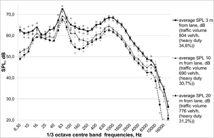
Table 1Low frequency SPL measured at noise barriers No. 1 and No. 2
1/3 octave band centre frequencies, Hz | 16 | 20 | 25 | 31.5 | 40 | 50 | 63 | 80 | 100 | 125 | 160 | 200 |
Noise barrier No. 1 | ||||||||||||
SPL 3 m from driving lane, dB | 62.6 | 61.3 | 60.2 | 60.1 | 62.1 | 68.1 | 71.7 | 65.9 | 65.4 | 66.8 | 64.4 | 64.1 |
SPL 4 m from noise barrier, dB | 58.6 | 57.0 | 56.2 | 55.5 | 56.7 | 59.2 | 64.8 | 58.7 | 53.5 | 52.0 | 46.8 | 44.8 |
Difference, dB | 4.0 | 4.3 | 4.1 | 4.7 | 5.3 | 8.9 | 6.8 | 7.1 | 11.9 | 14.8 | 17.6 | 19.3 |
Noise barrier No. 2 | ||||||||||||
SPL 3 m from driving lane, dB | 66.9 | 65.4 | 63.5 | 63.9 | 64.6 | 68.3 | 74.9 | 73.6 | 69.9 | 69.5 | 68.2 | 68.4 |
SPL 4 m from noise barrier, dB | 62.7 | 61.4 | 59.0 | 58.1 | 59.4 | 61.8 | 66.0 | 65.2 | 60.2 | 58.9 | 55.8 | 53.0 |
Difference, dB | 4.2 | 4.0 | 4.5 | 5.8 | 5.2 | 6.5 | 8.9 | 8.4 | 9.7 | 10.7 | 12.4 | 15.4 |
3.1. Equations, boundary conditions and initial values
To assign sound power level for linear sound source, the highest measured sound pressure level 3 m from driving lane was taken (72.5 dB at 63 Hz 1/3 octave band centre frequency) and calculated according to Eq. (1) and (2).
Linear noise source sound power levels were calculated according equations [6]. For cylindrical domain:
For ½ of cylindrical domain:
where: – Sound power level of linear source in dB per length unit, – Sound power level of linear source in W per length unit, – a distance to linear source, m.
Calculated sound power of linear source is 0.0002053 W/m. Boundary of ½ of cylinder was assigned as cylindrical wave radiation in a model. For definition of road surface Sound Hard Boundary conditions were selected. Grass covered ground surface has Impedance of 3 kPa·s·m−1 (according [7-8]) boundary conditions. All expressions of equations can be found in [9].
Considering that existing barriers have absorbing part as well as structure elements, the simplified model was designed to simulate acoustic field transformation influenced by absorbing material and sound – solid interaction. The noise barrier model was designed from 10 cm width macroscopic porous material part and 2 cm width solid part. Porous material (domain) modelled as an equivalent fluid, using empirical Delany-Bazley-Miki model [10, 11] with properties: flow resistivity – 20 kPa·s/m2, speed of sound and density values are taken from material (air properties). Noise barrier solid part – wood, with basic acoustic properties: 1150 kg/m3 density and 3500 m/s speed of sound. Within Comsol Acoustic-structure Interaction interface, fluid’s pressure loads solid domain, and the structural acceleration affects the fluid domain as a normal acceleration across the fluid-solid boundary [9]. All tops were modelled describing only as porous material.
Considering analysed frequencies and construction of modelled noise barriers, model mesh was calibrated for general physics, defining maximum element size 0.25 m, minimum element size 0.002 m, with maximum element growth rate 1.3. Parameters of mesh weren’t changed for different frequencies.
3.2. Results of acoustic simulation
It should be noted that SPL at low frequencies very depended (differs) on evaluation point place (height and distance from noise barrier), therefore to assess sound level reduction by enhancing noise barriers with different tops assessment at all spectrum (16-200 Hz) average sound pressure level was calculated at 4×9 m rectangle 4 m behind the noise barrier Figs. 2-3.
Table 2Simulation results of average SPL behind noise barrier, (in 4×9 m rectangle), dB
1/3 octave band centre frequencies, Hz | 16 | 20 | 25 | 31.5 | 40 | 50 | 63 | 80 | 100 | 125 | 160 | 200 | |
Free field SPL transformation | 79.9 | 78.9 | 77.9 | 76.8 | 75.7 | 74.7 | 73.7 | 72.6 | 71.5 | 70.6 | 69.4 | 68.4 | 86.4 |
Existing noise barrier | 79.7 | 78.5 | 76.8 | 74.5 | 71.4 | 68.7 | 66.7 | 64.4 | 60.8 | 59.8 | 56.7 | 54.7 | 84.3 |
Noise barrier with T top | 78.7 | 77.0 | 74.8 | 72.0 | 68.8 | 66.6 | 65.0 | 57.2 | 56.8 | 53.2 | 54.7 | 54.1 | 82.7 |
Noise barrier with 45º T top | 79.1 | 77.6 | 75.6 | 72.9 | 69.8 | 67.4 | 65.2 | 60.8 | 58.3 | 55.6 | 53.8 | 52.2 | 83.3 |
Noise barrier with quadratic top | 78.7 | 76.8 | 74.5 | 71.5 | 68.3 | 66.0 | 64.1 | 58.8 | 56.9 | 56.1 | 55.9 | 53.5 | 82.5 |
Noise barrier with octagon top | 78.9 | 77.1 | 74.8 | 71.9 | 68.9 | 66.3 | 64.4 | 59.5 | 56.9 | 55.9 | 54.0 | 52.1 | 82.8 |
Noise barrier with complex shape top | 78.8 | 77.0 | 74.6 | 71.7 | 68.5 | 66.2 | 63.9 | 57.9 | 56.6 | 54.4 | 54.6 | 52.9 | 82.7 |
Noise barrier with V top | 78.9 | 77.2 | 75.1 | 72.4 | 69.3 | 67.0 | 64.6 | 59.9 | 57.7 | 54.3 | 52.3 | 50.1 | 83.0 |
Examples of calculation in free field conditions, with simulated simplified existing noise barrier and enhanced noise barrier are presented in Fig. 3 (Appendix).
Fig. 2Simulated additional of averaged sound pressure level behind noise barrier by enhancing with additional top
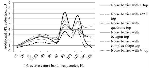
Numerical prediction results show that noise barrier enhancement by adding different tops gives 0.6-1.7 dB additional SPL reduction at 16-20 Hz frequency range, 1.3-3 dB additional SPL reduction at 15-63 Hz frequency range and 0.6-7.2 dB additional SPL reduction at 80-200 Hz frequency range. Different tops plays the best at different discrete frequencies, for example T top is most efficient at 80 Hz frequency and not effective at 200 Hz frequency, meanwhile effectiveness of V top is similar in all 80-200 Hz range.
4. Conclusions
Measurements results showed that that spectrum of heavy traffic busy road has 2 peaks of SPL: at 63 Hz and 800-1600 Hz frequencies. Measurements results also showed, that effectiveness of existing noise barriers are better in mid and high frequencies and less at low frequencies.
Numerical prediction showed that enhancement of existing noise barrier can improve effectiveness of noise barrier either at low frequencies. According calculation results, which where proceeded using finite element method, investigated tops can give such additional SPL reduction at low frequencies:
• 0.6-1.7 dB reduction at 16-20 Hz frequency range;
• 1.3-3 dB reduction at 15-63 Hz frequency range;
• 0.6-7.2 dB reduction at 80-200 Hz frequency range.
Looking to of simulation results at Table 2, the conclusion can be drawn that all investigated tops additionally reduces SPL at low frequencies by 1.0-1.8 dB however for discrete frequencies higher reduction can be achieved.
According to measurements results, regulated values and destination (reached to mitigate) frequencies various tops can be selected. In our case if we’d like to reduce noise at existing peak (SPL peak at 63 Hz frequencies) quadratic, octagon and complex shape tops would give best results.
References
-
Šaliūnas D., Volkovas V. Analysis of Assessments of Low Frequency Noise from Wind Turbines. Calculations of Impact Range According to HN 30:2009. Environmental Research, Engineering and Management, Vol. 63, Issue 1, 2013, p. 48-59.
-
Moller H., PedersenC. S. Low-frequency noise from large wind turbines. Journal of the Acoustical Society of America, Vol. 129, Issue 6, 2011, p. 3727-3744.
-
Kerstin P. W. Adverse effects of moderate levels of low frequency noise in the occupational environment. ASHRAE Transactions, Vol. 111, 2005, p. 672-683.
-
Venckus Ž., Grubliauskas R., Venslovas A. The research on the effectiveness of the inclined top type of a noise barrier. Journal of Environmental Engineering and Landscape Management, Vol. 20, Issue 2, 2012, p. 155-162.
-
Lithuanian Road Administration traffic intensity database, http://lakis.lakd.lt/vmpei/.
-
Bies D. A., Hansen C. H. Engineering Noise Control – Theory and Practice. Abingdon, Spon Press, Fourth Edition, 2009.
-
Embleton T. F. W., Piercy J. E., Daigle G. A. Effective flow resistivity of ground surfaces determined by acoustical measurements. Journal of the Acoustical Society of America, Vol. 74, Issue 4, 1983, p. 1239-1244.
-
Hutchins D. A., Jones H. W., Russell L. T. Model studies of acoustic propagation over finite impedance ground. Journal of Acta Acustica united with Acustica, Vol. 52, Issue 3, 1983, p. 169-178.
-
Comsol 4.4. Acoustics Module User’s Guide, 2011, p. 53.
-
Komatsu T. Improvement of the Delany-Bazley and Miki models for fibrous sound-absorbing materials. Journal of Acoustical Science and Technology, Vol. 29, Issue 2, 2008, p. 121-129.
-
Allard J. F., Atalla N. Propagation of Sound in Porous Media. Chichester, John Wiley and Sons, Ltd., 2009.
About this article

