A joint optimal policy of inspection and age based replacement based on a three-stage failure process

1. Introduction

Preventive maintenance (PM) and condition-based maintenance (CBM) are two popular maintenance policies in practice. Preventive maintenance, by which maintenance is implemented with a planned interval aiming at preventing potential failures from occurring, is still the most widely used policy in industry due to its easy implementation [1]. Nowadays CBM attracts more interest because of the efficiency of deriving the actual condition information [2].

Vibration data can express the condition of system exactly when operating. Through collecting and processing the vibration data, maintenance operators could make maintenance decisions on the basis of the actual condition obtained from inspection. Therefore, inspection is the foundation of implementing the PM and CBM policies as it can provide the information on the status of system checked to facilitate the determination and execution of repair and replacement decisions [3, 4]. Nowadays inspection based on vibration information has been widely applied in industry. Of course, inspection can be on-line or off-line. As to the off-line inspection, maintenance operators often inspect the system using hand-held inspection tools, such as SPM (Shock pulse method) instrument.

SPM has been widely used as a quantitative method in determining bearing health condition. Unlike vibration analysis that monitors a broad vibration band and then tries to isolate unique frequencies, SPM has developed a means to only “look” at the high frequency signals of rotating bearings [5, 6]. Through monitoring and analyzing high frequency shock waves generated by a bearing while rotating, SPM can provide a direct shock value indicating the bearing condition. The major benefit of SPM is providing a direct indication of bearing condition on a Green-Yellow-Red scale. Green means a good bearing, Yellow is a bearing with early damage and Red is more severe damage [7]. This is very important when monitoring installed bearings on machines for which there are no trends or comparable readings. Through years of application, SPM has been proven successfully as a diagnostic tool for bearings.

As maintenance operators inspect the bearings using SPM with a planned interval, the determination of inspection intervals is one of the key decisions. There are numerous PM models to determine the optimal inspection intervals [8, 9]. The delay-time concept, which assumes the state of system before failure to be either normal or defective, has obvious advantage for optimizing the inspection intervals because it can capture the relationship between inspection interval and number of failures [10]. Most importantly, numerous successful case studies have been published with actual applications in industry using delay-time concept [11-13].

However, the state of system may by described more than two before failure as three color scheme is mostly used to divide the state before failure into green (normal), yellow (need attention), and red (need immediate attention) in industrial applications [14]. For example, SPM divides the lifetime of bearings into three stages, namely normal, minor defective and severe defective, expressed by green, yellow and red respectively. Therefore, Wang firstly extended the two-stage delay time to a three-stage failure process, where the traditional failure delay time stage is further divided into two stages: minor defective stage and severe defective stage [15]. Finally a case study is presented to show that delaying maintenance is better than maintenance immediately and validate the efficiency of the proposed three-stage failure process. A preventive maintenance model with a two level inspection policy based on a three-stage failure process is proposed by Wang et al. [16]. Minor inspection and major inspection consist of the two-level inspection policy. Moreover, a planned PM is considered as maintenance window to prevent the occurrence of failure. Yang et al. [17, 18] developed imperfect inspection maintenance models based on a three-stage failure process. Monte Carlo simulation is used to present the efficiency of the three-stage failure process. An inspection optimization model based on a three-stage failure process is presented to optimize the shortening proportion of inspection interval when the minor defective stage is identified [19]. But age based replacement policy is not considered in [15-19].

Age based replacement policy is one of the most commonly used preventive maintenance and replacement policies. According to this policy, the system is replaced upon failure or at fixed age, whichever occurs first [20]. Preventive replacement is carried out to avoid unplanned downtime and higher failure loss, thus age based replacement policy is widely used to determine optimum preventive replacement time. The joint policy of regular inspections and age based preventive replacement has been widely used in industrial applications. Most researches have considered the age based preventive replacement policy [21-23], but joint optimization for inspection and replacement intervals based on the three-stage failure process has not been developed.

In this paper, a joint optimal policy of inspection and age based replacement based on a three-stage failure process is introduced. Both cases of perfect and imperfect inspections are considered. The system is replaced when it fails or reaches the certain age. Once the severe defective stage is identified, repair will be carried out. However, when the minor defective stage is identified, two options are assumed here for comparison: halving the subsequent inspection interval or repair it immediately. The long-run availability is used to jointly optimize the inspection and replacement intervals.

The remaining part of the paper is organized as follows. Section 2 introduces the modeling assumptions and notation. Section 3 provides the proposed availability models with imperfect inspection and perfect inspection case is modeled in Section 4. Section 5 presents a case study and Section 6 concludes the paper.

2. Modelling assumptions and notation

The following modeling assumptions and notation are presented for model building.

1) A single component system is considered, which only subject to a single failure mode.

2) The failure process of system is divided into three stages: normal stage $X_1$, minor defective stage $X_2$ and severe defective stage $X_3$. These three stages are assumed to be independent.

3) The system is subjected to inspection interval $t$ and age based replacement interval $T$. Age based replacement interval is a multiple of inspection interval as $T=Nt$ for simplicity.

4) Both perfect and imperfect inspection cases are considered. Perfect inspection can always reveal the defective stage no matter it is minor and severe. However, imperfect inspection may miss the minor defective stage with a probability of ($1-r$), but always can identify the severe defective stage.

5) If the system is found in the normal stage, do nothing.

6) On condition that the system is identified in the minor defective stage by an inspection, two options are assumed here, the first one is to shorten the subsequent inspection interval to be half of the current interval, and the other one is to repair immediately.

7) System is found to be in the severe defective stage, it is always repaired immediately.

8) Failure can be observed immediately and replacement is always carried out at once.

9) Replacement renews the system once the age of system reaches certain age $T$, which is an age limit of system.

10) Repair or replacement is regarded as renewing the system, though it may be the only option for a single component system.

3. Availability models with imperfect inspection

The availability models are formulated in this section to jointly optimize the inspection and age replacement intervals. The imperfect inspection case mainly means that an inspection may miss the minor defective stage with a probability of ($1-r$) but can always identify the severe defective stage. Fig. 1 presents the joint policy of imperfect inspection and age based replacement.

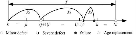
Fig. 1The system fails in i-1t,it before identifying any defective stages

Maximizing the availability is a main object of maintenance optimization. The decision objective is to derive the maximum long-run availability. Therefore, the long run expected renewal cycle downtime and length need to be derived firstly so that [24]:

According to the different decisions when the minor defective stage of system is identified depending on the assumption Eq. (6), two models are proposed.

3.1. Model 1

The system is renewed at failure, at the time of age based replacement and that a severe defect was first found prior to failure. However, if minor defective stage is identified, subsequent inspection intervals are halved.

3.1.1. The expected renewal cycle downtime

There exist three different kinds of renewal scenarios, namely failure renewal, inspection renewal caused by the identification of severe defective stage and age based replacement renewal. The downtime caused by these renewals in a renewal cycle consist the expected renewal cycle downtime, which will be introduced respectively.

3.1.1.1. The failure renewal scenarios

Failure renewal means the system fails in an inspection interval before identifying the severe defective stage or reaching the certain age $T$. However, according to the case whether the minor defective stage is identified by an inspection, there are two different failure renewals.

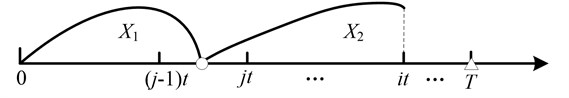
1) The system fails in $T_f$, $T_f\in \left(\right(i-1)t,it)$ before any defective stages are identified, as shown in Fig. 2. The minor defective stage starts in $\left(\left(j-1\right)t,jt\right)$ and ends in $\left(\left(i-1\right)t,it\right)$. All the inspections within $\left(jt,\left(i-1\right)t\right)$ miss the minor defective stage because of the imperfect inspection. The severe defective stage and failure happen within the same interval $\left(\left(i-1\right)t,it\right)$. The probability of such an event is given as:

2

$P\left(\right(i-1)t<T_f<it)$
$\mathrm{}\mathrm{}\mathrm{}\mathrm{}\mathrm{}\mathrm{}=P\left(\right(j-1)t<X_1<jt,(i-1)t-X_1<X_2<it-X_1,0<X_3<it-X_1-X_2)$
$\mathrm{}\mathrm{}\mathrm{}\mathrm{}\mathrm{}\mathrm{}=\sum _{j=1}^i{\int }_{(j-1)t}^{jt}{\int }_{\lambda \left(\right(i-1)t-x)}^{it-x}(1-r{)}^{i-j}{f}_{X_1}(x\left)f_{X_2}\right(y\left)F_{X_3}\right(it-x-y)dydx,$

where $i=$1, 2,…, $N$. Here we define $\lambda \left(x\right)=x$ if $x\ge 0$, otherwise $\lambda \left(x\right)=0$.

Fig. 2The system fails in i-1t,it before identifying any defective stages

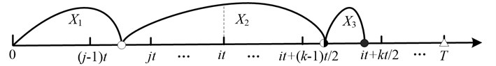
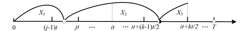
2) The system fails in $T_f$, $T_f\in (it+(k-1)t/2,it+kt/2)$ before identifying the severe defective stage by an inspection. The system degradates into minor defective stage within $\left(\left(j-1\right)t,jt\right)$. However, the minor defective stage is identified at $it$ and the subsequent inspection interval is halved, as depicted in Fig. 3. Similarly, the severe defective stage and failure happen within the same interval $\left(it+\left(k-1\right)t/2,it+kt/2\right)$. The probability of such a renewal is:

3

$P\left(it+\left(k-1\right)\frac{t}{2}<T_f<it+\frac{kt}{2}\right)$
$\mathrm{}\mathrm{}\mathrm{}\mathrm{}\mathrm{}\mathrm{}=P\left(\begin{array}{c}\left(j-1\right)t<X_1<jt,\\ it+\left(k-1\right)\frac{t}{2}-X_1<X_2<it+\frac{kt}{2}-X_1,\\ 0<X_3<it+\frac{kt}{2}-X_1-X_2\end{array}\right)$
$\mathrm{}\mathrm{}\mathrm{}\mathrm{}\mathrm{}\mathrm{}=\sum _{j=1}^i{\int }_{\left(j-1\right)t}^{jt}{f}_{X_1}\left(x\right){\int }_{it+\left(k-1\right)\frac{t}{2}-x}^{it+\frac{kt}{2}-x}{f}_{X_2}\left(y\right)(1-r{)}^{i-j}r{F}_{X_3}\left(it+\frac{kt}{2}-x-y\right)dydx.$

Fig. 3The system fails in it+k-1t/2,it+kt/2 after identifying minor defective stage at it

Therefore, the expected renewal cycle downtime due to failure renewal can be derived from Eqs. (2) and (3):

4

$E{D}_f\left(t\right)=\sum _{i=1}^N(D_f+(i-1\left)D_s\right)P\left(\right(i-1)t<T_f<it)$
$+\sum _{i=1}^{N-1}\sum _{k=1}^{2(N-i)}\left(D_f+\left(i+k-1\right)D_s\right)P\left(it+\left(k-1\right)\frac{t}{2}<T_f<it+\frac{kt}{2}\right).$

3.1.1.2. The inspection renewal scenarios

Inspection renewal occurs once the defective stages are identified. However, when the minor defective stage is identified, the subsequent inspection interval is halved. So the inspection renewal here only means the renewal caused by the identification of severe defective stage. Similarly, there are also two different renewals depending on whether the minor defective stage is identified.

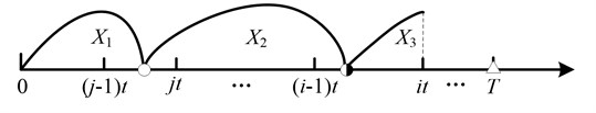
1) Fig. 4 shows the scenario that the system is renewed when the severe defective stage is found at $it$ before any minor defective stage is identified. The inspections miss the minor defective stage $\left(i-j\right)$ times. So the probability of such an inspection renewal is:

5

$P(T_{ps}=it)=P\left(\right(j-1)t<X_1<jt,(i-1)t-X_1<X_2<it-X_1,X_3>it-X_1-X_2)$
$\mathrm{}\mathrm{}\mathrm{}\mathrm{}\mathrm{}\mathrm{}=\sum _{j=1}^i{\int }_{(j-1)t}^{jt}{f}_{X_1}\left(x\right){\int }_{\lambda \left(\right(i-1)t-x)}^{it-x}{f}_{X_2}\left(y\right)(1-r{)}^{i-j}(1-F_{X_3}(it-x-y))dydx.$

Fig. 4The system renews at it before any minor defective stage is identified

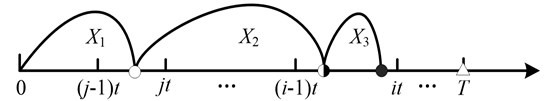
2) Fig. 5 presents the scenario that inspection renewal occurs at $it+kt/2$ when the minor and severe defective stages are identified at $it$ and $it+kt/2$ respectively. The inspections within $\left(jt,\left(i-1\right)t\right)$ miss the minor defective stage but identify it at $it$ and then the subsequent inspection interval is halved:

6

$P\left(T_{ps}=it+\frac{kt}{2}\right)$
$\mathrm{}\mathrm{}\mathrm{}\mathrm{}\mathrm{}\mathrm{}=P\left(\begin{array}{c}\left(j-1\right)t<X_1<jt,\\ it+\frac{\left(k-1\right)t}{2}-X_1<X_2<it+\frac{kt}{2}-X_1,\\ X_3>it+\frac{kt}{2}-X_1-X_2\end{array}\right)$
$\mathrm{}\mathrm{}\mathrm{}\mathrm{}\mathrm{}\mathrm{}=\sum _{j=1}^i{\int }_{\left(j-1\right)t}^{jt}{f}_{X_1}\left(x\right){\int }_{it+\frac{\left(k-1\right)t}{2}-x}^{it+\frac{kt}{2}-x}{f}_{X_2}\left(y\right)(1-r{)}^{i-j}r\left(1-F_{X_3}\left(it+\frac{kt}{2}-x-y\right)\right)dydx.$

Fig. 5The system renews at it+kt/2 after the minor defective stage is identified at it

Then the expected renewal cycle downtime of an inspection renewal can be derived using Eqs. (5) and (6) as:

7

$E{D}_s\left(t\right)=\sum _{i=1}^{N-1}\left(D_{ps}+i{D}_s\right)P\left(T_{ps}=it\right)+\sum _{i=1}^{N-1}\sum _{k=1}^{2\left(N-i\right)-1}\left(D_{ps}+\left(i+k\right)D_s\right)P\left(T_{ps}=it+\frac{kt}{2}\right).$

3.1.1.3. The age based replacement renewal scenarios

The system is renewed once it reaches certain age $T$ according to the assumption Eq. (9). There are also two scenarios.

1) The age based replacement renewal is happened before any defective stages are identified. However, there may exist three possible scenarios, see Fig. 6. Firstly, the normal stage $X_1$ exceeds the age $T$. Secondly, the normal stage ends within $\left(\left(j-1\right)t,jt\right)$. The minor defective stage is longer than $T-X_1$ but missed by inspections. Finally, the minor defective stage starts within $\left(\left(j-1\right)t,jt\right)$, ends in $\left(\left(N-1\right)t,T\right)$ but all missed. The severe defective stage is longer than $T-X_1-X_2$. The probability of such a renewal is:

8

$P\left(T_{r1}=Nt\right)=P(X_1>Nt)+P\left(\right(j-1)t<X_1<jt,X_2>Nt-X_1)$
$\mathrm{}\mathrm{}\mathrm{}\mathrm{}\mathrm{}+P\left(\left(j-1\right)t<X_1<jt,\left(N-1\right)t-X_1<X_2<Nt-X_1,X_3>Nt-X_1-X_2\right)$
$={\int }_{Nt}^{\mathrm{\infty }}{f}_{X_1}\left(x\right)dx+\sum _{j=1}^N{\int }_{\left(j-1\right)t}^{jt}(1-r{)}^{N-j}{f}_{X_1}(x\left)\right(1-F_{X_2}(Nt-x))dx$
$\mathrm{}\mathrm{}\mathrm{}\mathrm{}\mathrm{}\mathrm{}+\sum _{j=1}^N{\int }_{\left(j-1\right)t}^{jt}(1-r{)}^{N-j}{f}_{X_1}(x){\int }_{\left(N-1\right)t-x}^{Nt-x}{f}_{X_2}\left(y\right)\left(1-F_{X_3}\left(Nt-x-y\right)\right)dydx.$

Fig. 6The system renews at age T before any defective stages are identified

2) The system renews at age $T$ after the minor defective stage is found at $it$. There also exist two different scenarios, see Fig. 7. Firstly, The normal stage ends in $\left(\left(j-1\right)t,jt\right)$ but the minor defective stage is longer than $T-X_1\text{.}$ The second is the minor defective stage ends in $\left(\left(N-1\right)t+t/2,T\right)$ and the severe defective stage exceeds the length of $T-X_1-X_2$. All the inspections between $jt$ and $\left(i-1\right)t$ miss the minor defective stage in both scenarios:

9

$P\left(T_{r2}=Nt\right)=P\left(\right(j-1)t<X_1<jt,X_2>Nt-X_1)$
$+P\left(\right(j-1)t<X_1<jt,(N-1)t+\frac{t}{2}-X_1<X_2<Nt-X_1,X_3>Nt-X_1-X_2$
$=\sum _{j=1}^i{\int }_{(j-1)t}^{jt}{f}_{X_1}\left(x\right)(1-r{)}^{i-j}r(1-F_{X_2}(Nt-x))dx$
$+\sum _{j=1}^i{\int }_{(j-1)t}^{jt}{f}_{X_1}\left(x\right)(1-r{)}^{i-j}r{\int }_{(N-1)t+\frac{t}{2}-x}^{Nt-x}{f}_{X_2}\left(y\right)(1-F_{X_3}(Nt-x-y\left)\right)dydx.$

Fig. 7The system renews at age T after identifying the minor defective stage at it

The expected renewal cycle downtime of age based replacement renewal can be derived from Eqs. (8) and (9) as:

10

$E{D}_r\left(t\right)=\left(\left(N-1\right)D_s+D_r\right)P\left(T_{r1}=Nt\right)+\sum _{i=1}^{N-1}\left(\left(2N-i-1\right)D_s+D_r\right)P\left(T_{r2}=Nt\right).$

3.1.2. The expected renewal cycle length

These three kinds of expected renewal cycle length can be derived according to the three different renewal scenarios.

3.1.2.1. The failure renewal scenarios

In order to derive the expected cycle length of failure renewal, the pdf of failure needs to be formulated. Firstly, if the system fails in $\left(\left(i-1\right)t,it\right)\text{,}$ the pdf of failure at $T_f\text{,}$$T_f\in \left(\right(i-1)t+z,(i-1)t+z+dz)$, $z\in (0,t)$ can be derived from Eq. (2) as:

11

$P\left(\left(i-1\right)t+z<T_f<\left(i-1\right)t+z+dz\right)$
$\mathrm{}\mathrm{}\mathrm{}\mathrm{}\mathrm{}\mathrm{}=\sum _{j=1}^i{\int }_{(j-1)t}^{jt}{\int }_{\lambda \left(\right(i-1)t-x)}^{(i-1)t+z-x}(1-r{)}^{i-j}{f}_{X_1}(x\left)f_{X_2}\right(y\left)f_{X_3}\right((i-1)t+z-x-y)dydxdz.$

Similarly, the pdf of failure at $T_f$, $T_f\in (it+(k-1)t/2+z,it+(k-1)t/2+z+dz)$, $z\in (0,t/2)$ can be derived from Eq. (3) as:

12

$P\left(it+\left(k-1\right)\frac{t}{2}+z<T_f<it+\left(k-1\right)\frac{t}{2}+z+dz\right)$
$\mathrm{}\mathrm{}\mathrm{}\mathrm{}\mathrm{}\mathrm{}=\sum _{j=1}^i{\int }_{(j-1)t}^{jt}{f}_{X_1}\left(x\right){\int }_{it+(k-1)\frac{t}{2}-x}^{it+(k-1)\frac{t}{2}+z-x}{f}_{X_2}\left(y\right)(1-r{)}^{i-j}r{f}_{X_3}\left(it+(k-1)\frac{t}{2}\right.$
$\mathrm{}\mathrm{}\mathrm{}\mathrm{}\mathrm{}\mathrm{}+z-x-y)dydxdz.$

Accordingly, the expected renewal cycle length caused by failure renewal is expressed as:

13

$E{L}_f\left(t\right)=\sum _{i=1}^N{\int }_0^t((i-1)t+z\left)P\right((i-1)t+z<T_f<(i-1)t+z+dz)$
$+\sum _{i=1}^{N-1}\sum _{k=1}^{2\left(N-i\right)}{\int }_0^{\frac{t}{2}}\left(it+\left(k-1\right)\frac{t}{2}\mathrm{}+z\right)P\left(it+\left(k-1\right)\frac{t}{2}\mathrm{}+z<T_f\right.<it$
$\left.\mathrm{}\mathrm{}\mathrm{}\mathrm{}\mathrm{}\mathrm{}+\left(k-1\right)\frac{t}{2}+z+dz\right).$

3.1.2.2. The inspection renewal scenarios

The expected renewal cycle length caused by an inspection renewal is given as:

14

$E{L}_s\left(t\right)=\sum _{i=1}^{N-1}itP\left(T_{ps}=it\right)+\sum _{i=1}^{N-1}\sum _{k=1}^{2\left(N-i\right)-1}\left(it+\frac{kt}{2}\right)P\left(T_{ps}=it+\frac{kt}{2}\right).$

3.1.2.3. The age replacement renewal scenarios

The expected renewal cycle length of age based replacement renewal is:

15

$E{L}_r\left(t\right)=NtP\left(T_{r1}=Nt\right)+\sum _{i=1}^{N-1}NtP\left(T_{r2}=Nt\right).$

3.1.3. The long-run availability

Based on the different expected renewal cycle downtime and length, the long-run availability is given using the renewal theorem [25], as shown in Eq. (16):

16

$A\left(T\right)=\frac{E{L}_f\left(T\right)+E{L}_s\left(T\right)+E{L}_r\left(T\right)}{E{D}_f\left(T\right)+E{D}_s\left(T\right)+E{D}_r\left(T\right)+E{L}_f\left(T\right)+E{L}_s\left(T\right)+E{L}_r\left(T\right)}.$

3.2. Model 2

The system is replaced at the time of defect identification no matter it is minor or major prior to failure. The system is also renewed at failure and at the time of age based replacement.

In model 2, there also exist three kinds of renewals, namely failure renewal, age based replacement renewal and inspection renewal. However, inspection renewal may be caused by the identification of minor or severe defective stage, which is different from model 1. The expected renewal cycle downtime and length are derived as follows.

3.2.1. The expected renewal cycle downtime

3.2.1.1. The failure renewal scenarios

As the system is renewed at the time of the identification of two defective stages, failure only happens in the same interval before any defective stages are found. Therefore, the probability of failure renewal is same to the Eq. (2). The expected downtime of failure renewal can be derived as:

17

$E{D}_f\left(t\right)=\sum _{i=1}^N\left(D_f+\left(i-1\right)D_s\right)P\left(\left(i-1\right)t<T_f<it\right)=\sum _{i=1}^N\sum _{j=1}^i(D_f$
$\mathrm{}\mathrm{}\mathrm{}\mathrm{}\mathrm{}\mathrm{}+(i-1)D_s){\int }_{\left(j-1\right)t}^{jt}{\int }_{\lambda \left(\left(i-1\right)t-x\right)}^{it-x}(1-r{)}^{i-j}{f}_{X_1}(x\left)f_{X_2}\right(y\left)F_{X_3}\right(it-x-y)dydx.$

3.2.1.2. The inspection renewal scenarios

The inspection renewal may be carried out once the defective stages are identified no matter it is minor or severe. Therefore, two different renewal scenarios are considered.

1) The system is renewed at it when the severe defective stage is found firstly before the minor defective stage is identified. The probability of this scenario is same to the Eq. (5). Thus the expected renewal cycle downtime of this scenario is:

18

$E{D}_s\left(t\right)=\sum _{i=1}^{N-1}\left(D_{ps}+i{D}_s\right)P\left(T_{ps}=it\right)$
$\mathrm{}\mathrm{}\mathrm{}\mathrm{}\mathrm{}\mathrm{}=\sum _{i=1}^{N-1}\sum _{j=1}^i(D_{ps}+i{D}_s){\int }_{\left(j-1\right)t}^{jt}{f}_{X_1}\left(x\right){\int }_{\lambda \left(\left(i-1\right)t-x\right)}^{it-x}{f}_{X_2}\left(y\right)(1-r{)}^{i-j}(1-F_{X_3}(it$
$\mathrm{}\mathrm{}\mathrm{}\mathrm{}\mathrm{}\mathrm{}-x-y\left)\right)dydx.$

2) The system is renewed at it when the minor defective stage is found firstly prior to failure, see Fig. 8. All the inspections between $\left(\left(j-1\right)t,it\right)$ miss the minor defective stage. The probability of such a scenario is:

19

$P(T_{pm}=it)=P\left(\right(j-1)t<X_1<jt,X_2>it-X_1)$
$\mathrm{}\mathrm{}\mathrm{}\mathrm{}\mathrm{}\mathrm{}=\sum _{j=1}^i{\int }_{(j-1)t}^{jt}{f}_{X_1}\left(x\right)(1-r{)}^{i-j}r(1-F_{X_2}(it-x))dx.$

Fig. 8The system renews at it when the minor defective stage is identified

Accordingly, the expected renewal cycle downtime of this renewal is:

20

$E{D}_m\left(t\right)=\sum _{i=1}^{N-1}\left(D_{pm}+i{D}_s\right)P\left(T_{pm}=it\right)$
$\mathrm{}\mathrm{}\mathrm{}\mathrm{}\mathrm{}\mathrm{}=\sum _{i=1}^{N-1}\sum _{j=1}^i(D_{pm}+i{D}_s){\int }_{(j-1)t}^{jt}{f}_{X_1}\left(x\right)(1-r{)}^{i-j}r(1-F_{X_2}(it-x))dx.$

3.2.1.3. The age replacement renewal scenarios

The probability of this scenario is the same to the Eq. (8). Thus the expected renewal cycle downtime of this event is given as:

21

$E{D}_r\left(t\right)=\left(\right(N-1)D_s+D_r)P(T_{r1}=Nt)=\left(\right(N-1)D_s+D_r)\left({\int }_{Nt}^{\mathrm{\infty }}{f}_{X_1}\left(x\right)dx\right.$
$\mathrm{}\mathrm{}\mathrm{}\mathrm{}\mathrm{}\mathrm{}+\sum _{j=1}^N{\int }_{\left(j-1\right)t}^{jt}(1-r{)}^{N-j}{f}_{X_1}(x\left)\right(1-F_{X_2}(Nt-x))dx$
$\left.\mathrm{}\mathrm{}\mathrm{}\mathrm{}\mathrm{}\mathrm{}+\sum _{j=1}^N{\int }_{(j-1)t}^{jt}(1-r{)}^{N-j}{f}_{X_1}(x){\int }_{(N-1)t-x}^{Nt-x}{f}_{X_2}\left(y\right)(1-F_{X_3}(Nt-x-y\left)\right)dydx\right).$

3.2.2. The expected renewal cycle length

Similarly, three different renewal scenarios should be considered in order to derive the expected renewal cycle length.

3.2.2.1. The failure renewal scenarios

The system fails in an inspection interval before any defective stage is identified. The pdf of such a renewal is similar to Eq. (11). So the expected cycle length of this failure renewal is given by:

22

$E{L}_f\left(t\right)=\sum _{i=1}^N{\int }_0^t((i-1)t+z\left)P\right((i-1)t+z<T_f<(i-1)t+z+dz)$
$\mathrm{}\mathrm{}\mathrm{}\mathrm{}\mathrm{}\mathrm{}=\sum _{i=1}^N\sum _{j=1}^i{\int }_0^t{\int }_{(j-1)t}^{jt}{\int }_{\lambda \left(\right(i-1)t-x)}^{(i-1)t+z-x}\left(\right(i-1)t+z)(1-r{)}^{i-j}{f}_{X_1}(x\left)f_{X_2}\right(y\left)f_{X_3}\right((i-1)t$
$\mathrm{}\mathrm{}\mathrm{}\mathrm{}\mathrm{}\mathrm{}+z-x-y)dydxdz$

3.2.2.2. The inspection renewal scenarios

The expected cycle length of an inspection renewal caused by the identification of severe defective stage is:

23

$E{L}_s\left(t\right)=\sum _{i=1}^{N-1}itP\left(T_{ps}=it\right)$
$\mathrm{}\mathrm{}\mathrm{}\mathrm{}\mathrm{}\mathrm{}=\sum _{i=1}^{N-1}\sum _{j=1}^{i}it{\int }_{(j-1)t}^{jt}{f}_{X_1}\left(x\right){\int }_{\lambda \left(\right(i-1)t-x)}^{it-x}{f}_{X_2}\left(y\right)(1-r{)}^{i-j}(1-F_{X_3}(it-x-y))dydx.$

Moreover, the expected cycle length of an inspection renewal caused by the identification of minor defective stage is given as:

24

$\begin{array}{c}E{L}_m\left(t\right)=\sum _{i=1}^{N-1}itP(T_{pm}=it)\end{array}$
$\mathrm{}\mathrm{}\mathrm{}\mathrm{}\mathrm{}\mathrm{}=\sum _{i=1}^{N-1}\sum _{j=1}^{i}it{\int }_{(j-1)t}^{jt}{f}_{X_1}\left(x\right)(1-r{)}^{i-j}r(1-F_{X_2}(it-x))dx.$

3.2.2.3. The age replacement renewal scenarios

The expected renewal cycle length of age based replacement renewal is given by:

25

$E{L}_r\left(t\right)=NtP\left(T_{r1}=Nt\right)=Nt\left({\int }_{Nt}^{\mathrm{\infty }}{f}_{X_1}\left(x\right)dx\right.$
$\mathrm{}\mathrm{}\mathrm{}\mathrm{}\mathrm{}\mathrm{}+\sum _{j=1}^N{\int }_{(j-1)t}^{jt}(1-r{)}^{N-j}{f}_{X_1}(x\left)\right(1-F_{X_2}(Nt-x))dx$
$\left.\mathrm{}\mathrm{}\mathrm{}\mathrm{}\mathrm{}\mathrm{}+\sum _{j=1}^N{\int }_{(j-1)t}^{jt}(1-r{)}^{N-j}{f}_{X_1}(x){\int }_{(N-1)t-x}^{Nt-x}{f}_{X_2}\left(y\right)(1-F_{X_3}(Nt-x-y\left)\right)dydx\right).$

3.2.3. The long-run availability

In the similar way as Eq. (16), the long-run availability of model 2 is expressed as:

26

$A\left(T\right)=\frac{E{L}_f\left(T\right)+E{L}_s\left(T\right)+E{L}_m\left(T\right)+E{L}_r\left(T\right)}{E{D}_f\left(T\right)+E{D}_s\left(T\right)+E{D}_m\left(T\right)+E{D}_r\left(T\right)+E{L}_f\left(T\right)+E{L}_s\left(T\right)+E{L}_m\left(T\right)+E{L}_r\left(T\right)}.$

4. Availability models with perfect inspection

The case of imperfect inspection has been presented in Section 3. Perfect inspection means inspection can always reveal the state of system. The defective stage will be found immediately once it occurs no matter it is minor or severe. Similarly, three different renewal scenarios are considered, namely failure renewal, age based replacement renewal and inspection renewal with the identification of minor or severe defective stage. The availability model with perfect inspection follows the same principle as the imperfect inspection case. Therefore, the derivation of renewal probabilities with perfect inspection will be left to Appendix.

5. Case study

A case study is presented in this section to demonstrate the efficiency of the proposed models and derive the optimal inspection and replacement intervals.

5.1. Wind turbine gearbox experiment

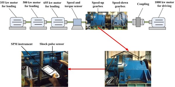
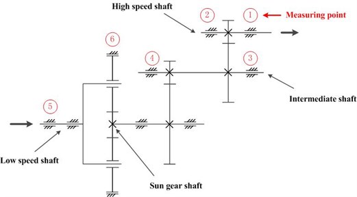
The experimental system used in this paper mainly concentrates on the bearings condition inspection of wind turbines. The gearbox of industrial wind turbine is inspected aperiodically by SPM instrument, as shown in Fig. 9. The system includes two gearboxes, one is speed-down gearbox, other is speed-up gearbox. Four motors are used, a 1000 kw for driving the gearboxes and three motors for loading with power 355 kw, 500 kw and 655 kw respectively. A speed and torque sensor is to measure the rotating speed. The speed-up gearbox is the test gearbox. In the test gearbox, the ring gear is stationary, a sun gear rotates around a fixed center, and planet gears not only rotate around their own centers but also revolve around the center of the sun gear. The planet gears mesh simultaneously with both the sun gear and the ring gear. The inner structure of the test gearbox and measuring points of SPM sensor are depicted as Fig. 10.

Fig. 9The gearbox test rig of FL600 wind turbine

The maintenace data we collected include threefolds: the time that the bearings starts to operate; the time that the bearings are replaced because of the identified defect, age replacement or failure; the time that last inspection before renewal or replacement.

After a period of experiment, the maintenance data of bearings are collected, as shown in Table 1.

Table 1The renewal data of rolling bearings

Start time	Happen time	Minor defect	Severe defect	Age replacement	Failure	Length	Inspection time
0	219	√				219	194
325	370	√				45	21
398	413		√			15	0
459	497			√		38	17
518	717	√				199	149
727	785		√			58	29
801	878	√				77	54
883	924			√		41	26
939	952		√			13	0
965	1022	√				57	28
1037	1109				√	72	42
1112	1407	Normal when the inspection is ended				283

Fig. 10The test gearbox and measuring points location

5.4. Maintenance decision-making

Depending on the given distribution and downtime parameters, we can determine the optimal decision variables and analyze the outputs of the proposed models.

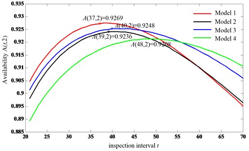
As for the availability models with imperfect inspection in Section 3, Figs. 11 and 12 show the results of the two proposed models in terms of the inspection and replacement intervals. In model 1 (halving the subsequent inspection intervals when the minor defect is identified with imperfet inspection), the optimal intervals are $t^{*}=$37, $N^{*}=$2 with maximum long-run availability $A^{*}$(37, 2)$=$0.9269. However, the optimal intervals are $t^{*}=$39, $N^{*}=$ 2 with maximum long-run availability $A^{*}$(39, 2) $=$0.9236 in model 2 (repair immediately when the minor defect is identified with imperfet inspection).

On the other hand, the results of the availability models with perfect inspection case in terms of the two decision variables are presented in Figs. 13 and 14. The optimal intervals are $t^{*}=$40, $N^{*}=$ 2 with maximum long run availability $A^{*}$(40, 2)$=$0.9248 in model 3 (halving the subsequent inspection intervals when the minor defect is identified with perfet inspection). But the optimal solutions are $t^{*}=$48, $N^{*}=$ 2 with maximum long run availability $A^{*}$(48, 2) $=$0.9208 in model 4 (repair immediately when the minor defect is identified with perfet inspection).

Fig. 11The long-run availability of the model 1 with imperfect inspection

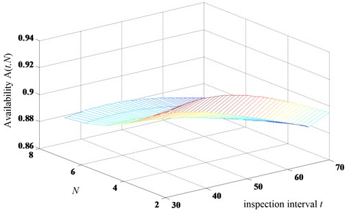
Fig. 12The long-run availability of the model 2 with imperfect inspection

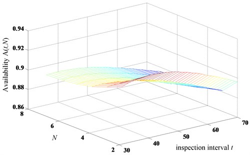
Fig. 13The long-run availability of the model 3 with perfect inspection

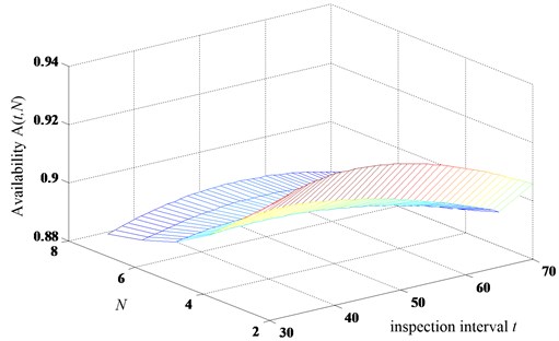
Fig. 15 presents the results of the four proposed models for comparison. As all of the optimal $N$ of four models are 2, Fig. 15 gives the availability values with constant $N=$2 and different inspection intervals $t$.

From the results, we can see that the optimal availability value of model 1 is larger than model 2 under the imperfect inspection case. The same results can be derived under the perfect inspection case. It shows that no matter the perfect inspection or not, the models 1 and 3 is optimal compared with models 2 and 4 with the given parameters from the numerical examples. The results mean that shortening the inspection interval is better than replacing immediately regarding the maximum long-run availability under the joint policy of inspection and age replacement. The results also shows the efficiency and importance of delaying the maintenance action based on the three-stage failure process. Therefore, when the minor defective stage is identified, the optimal action is to shortening the subsequent inspection interval for these systems subject to three-stage failure process. This conclusion can help the managers make scientific maintenance decisions.

Fig. 14The long-run availability of the model 4 with perfect inspection

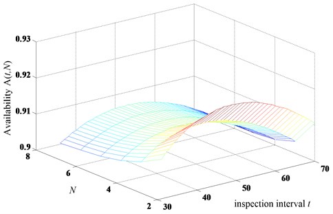
Fig. 15The comparison of the four models

6. Conclusions

Regular inspections and age based preventive replacement are common activities in industrial maintenance actions. In this paper, a joint optimal policy of inspection and age based replacement for a single component based on a three-stage failure process is proposed aiming at jointly optimizing the inspection and replacement intervals. The objective is the maximum long-run availability. Three states of system are divided before failure by the concept of three-stage failure process, namely normal, minor defective and severe defective. Age based replacement policy is also considered due to its wide applications in industry. The system is replaced when it fails or reaches certain age. Once the severe defective stage is identified, maintenance action is carried out. Two different models are proposed according to the different measures of identifying the minor defective stage. A case study is presented to demonstrate the efficiency of the proposed models. The results show that delaying the maintenance action is better than replacing immediately based on the three-stage failure process with this joint maintenance policy.

Further research with the concept of three-stage failure process can be developed such as: 1) The complex or multi-component system which are more commom in practice can be considered, 2) The combination of condition-based maintenance and the concept of three-stage failure process should be considered as the identification of the three stages will be easier with condition-based maintenace policy. These issues will be researched in the future.