Application of alpha-stable distribution approach for local damage detection in rotating machines

1. Introduction

Local damage detection in complex heavy-duty mechanical systems as belt conveyor drive systems is a very challenging problem [1, 2]. Analysis of vibration signal acquired on the housing is the most effective way to evaluate condition of the bearings/gears. Due to complex structure of mechanical system and consequently many non-informative (in the analysed context) sources of measured vibration, signal contains many different components. In order to detect presence of fault based on measured vibration, an extraction informative signal from raw, noisy observation is the key issue. In other words, the signal has to be decomposed into the informative and non-informative parts [1-3]. In the literature one can find several methods that use properties of the signal (impulsiveness, cyclicity, periodicity, etc.) to evaluate informativenes of the signal. It might happen in complex mechanical systems, that there are several co-existing informative bands due to existing resonances and anti-resonances of the structure. Consequently, one might notice in practice that different frequency bands of the considered signal might carry different level of diagnostic information. Thus it is of high importance to divide the frequency spectrum of the signal into sub-bands to assess each one and quantify its diagnostic informativeness. As mentioned, the informativeness might be quantified by using many different approaches.

In the literature one can find methods of local damage detection that are based on enhancement (denoising) of signal using hidden/included determinism related to rotation of elements or predictable behaviour of particular spectral components i.e. time domain signal averaging [4] or deterministic component removal using adaptive filters [5-9]. However, signal from machine with local damage is very non-stationary therefore it is well known that in many cases time- frequency methods are more appropriate [10-20].

Other approach is based on informative band selection that is basis for filtering procedure. It can be simple band pass filter (filtering around mesh, resonance freq. etc.) [3, 21], set of filters (filterbank, i.e. kurtogram) [3, 22] or more advanced amplitude characteristic of the filter that will maximize: impulsivity of the extracted signal [3, 21, 22] or impulsivity in given frequency bin/band [23-26] or even specific structure of envelope spectrum [26]. An important class of techniques is time-frequency methods. They are very suitable to analyse non-stationary signals with time varying structure [12-18, 27]. A natural approach is to exploit cyclostationarity of the signal [28]. Signal from damaged bearings/gearbox is nonstationary, due to its cyclic nature it might be considered as cyclostationary. Advantages of such approach were summarised by Antoni [29]. A generalization of signal component modulation was introduced by Urbanek [30]. Other recent works are based on local maxima method [16], sparsity [31-33] or statistical measures based on moments, quantiles, or cumulative distribution functions [34] and stochastic modelling [34-39].

In this paper we extend somehow the idea of spectral kurtosis and proposed recently set of more robust selectors. However, we do not calculate simple statistic for set of sub-signals obtained by decomposition of raw data by using filter-bank (spectrogram) but we model the distribution of each sub-signal. Because the sub-signals corresponding to informative frequency bins exhibit impulsive nature then we propose to model them by using a $\alpha$-stable distribution. This distribution is an extension of the classical Gaussian one [40]. The stable distributions are especially important in the context of modelling of data with visible jumps but it should be mentioned that for $\alpha$ parameter equal to 2 the $\alpha$-stable distribution reduces to Gaussian one. Therefore they can be used also for sub-signals of healthy machine or not related to informative frequency band. For each sub-signal (corresponding to each frequency bin) we fit the stability parameter of the $\alpha$-stable distribution, i.e. the $\alpha$ parameter. Finally, we obtain distribution of the stability parameter versus frequency, that provides similar picture as spectral kurtosis but type of selector is different. Moreover, we also analyse measures of dependence for each sub-signal. However, it should be said that classical measure such as autocovariance (or autocorrelation) is not properly defined for processes with infinite second moment (for instance for processes based on the $\alpha$-stable distribution) [40], so alternative measures of dependence should be considered here. In this paper we analyse two of them, namely an autocovariation and autocodifference. Visualization of autocovariation and autocodifference functions for each sub-signal results in new form of time-frequency map that presents diagnostic information in very clear way.

The paper is organized as follows. In Section 2 we present in details methodology related to informative frequency band selection for local damage detection. This algorithm incorporates short time Fourier transform, sub-signals extraction, creation of new time-frequency maps based on the autocovariation and autocodifference and finally fitting an $\alpha$-stable distribution to appropriate sub-signals. In Section 3 we present analysis of a simulated signal in the context of the presented methodology while in Section 4 we examine the real data set. The last section contains conclusion.

2. Methodology

In this section we describe in details the new method that can be used for selection of the informative frequency band (IFB) and local damage detection. The proposed algorithm is an extension of the classical methodology based on the spectral kurtosis [24]. The spectral kurtosis is the characteristic of the signal calculated according to the frequencies in time-frequency representation (spectrogram). More precisely, in this methodology first the raw signal is transformed into the time-frequency map through the short-time Fourier transform (STFT) [41]. The STFT is defined as:

where $w(t-\tau )$ is the shifted window and $x_k$ is the input signal ($k=$ 0, 1, 2,…, $N-1$). Each sub-signal corresponding to appropriate frequencies can be treated as a time series. It is worth to mention that window width and number of samples overlapping affect quality of results. Since the STFT matrix is complex, absolute value needs to be taken to obtain the spectrogram. After this transformation in the classical approach for each sub-signal from the spectrogram corresponding to appropriate $f\in F$ the statistic called kurtosis is calculated. The empirical kurtosis for vector of observations $x_1$, $x_2$,…, $x_N$ has the following form:

Instead of the kurtosis the other statistics (selectors) can be calculated in order to find the IFB. We only mention here two of them like the Jacque-Berra or Kolmogorov-Smirnov statistics, [25, 34].

Generally, the mentioned selectors are constructed under the assumption: distribution of sub-signal corresponding to healthy condition should be closer to Gaussian in comparison to distribution of sub-signal corresponding to damage condition (IFB, because of the impulsive nature of those sub-signals). An approach proposed here could be considered as a step forward in this field. It is suggested to analyze the sub-signals corresponding to frequency bands in the context of an $\alpha$-stable distribution approach (instead of Gaussian distribution). An $\alpha$-stable distribution is very often treated as a natural extension of the classical Gaussian one. The stable distributions are especially important in the context of modelling of data with visible jumps but it should be mentioned that for $\alpha$ parameter equal to 2 the $\alpha$-stable distribution reduces to Gaussian one.

In the proposed procedure, we treat the sub-signals corresponding to appropriate frequencies as samples from $\alpha$-stable distribution, since we expect a set of impulses (in statistical meaning – a set of extreme values) in a damaged gear case and the $\alpha$-stable distribution can perfectly exhibit such behaviour. We mention that a random variable $X$ is an $\alpha$-stable distributed if its characteristic function takes the following form:

where $\alpha$$(0<\alpha \le 2)$ is stability parameter, $\beta (-1\le \beta \le 1)$ is asymmetry parameter, $\sigma$$(\sigma >0)$ is scale parameter and $\mu$$(\mu \in R)$ is location parameter. The α-stable distributed random variable has ‘heavy’ tails, i.e. its cumulative probability density function decays with power law. Therefore, there is a high probability of the variable having extreme values, which is useful in modelling of impulsive signal.

In our procedure by the assumption that the sub-signals are described by the $\alpha$-stable distribution, in the next step for each time series corresponding to appropriate frequencies we estimate the $\alpha$ parameter. In the literature one can find different estimation methods that can be used here [42-44]. In this paper we apply the regression method which is based on the characteristic function of the considered distribution Eq. (3).

Despite many advantages of $\alpha$-stable distribution it has one significant disadvantage. Namely, except $\alpha$ equal to 2, for the $\alpha$-stable distributed random variables the variance is infinite, therefore for models or processes based on this distribution the classical measure of dependence such as autocovariance (or autocorrelation) is not properly defined. However, for processes with infinite second moment and finite first moment (i.e. $\alpha$-stable with $\alpha >1$), alternative measures of dependence are considered. In this paper we analyze two of them, namely an autocovariation and autocodifference. The autocovariation for signal $X\left(t\right)$ is defined as [45]:

where $S_t=\mathrm{s}\mathrm{i}\mathrm{g}\mathrm{n}\left(X\right(t\left)\right)$. For vector of observations $x_1$, $x_2$,…, $x_N$ the sample autocovariation is given by [45]:

where $l=\mathrm{m}\mathrm{a}\mathrm{x}(1,1+k)$ and $r=\mathrm{m}\mathrm{i}\mathrm{n}(N,N+k)$ and $s_t=\mathrm{s}\mathrm{i}\mathrm{g}\mathrm{n}\left(x_t\right)$.

Another measure of dependence that can be used for $\alpha$-stable models is called autocodifference [46]. It is defined through the characteristic function in the following way:

Its sample version is defined as [46]:

where:

is the empirical characteristic function calculated for vector of observations $x_1$, $x_2$,…, $x_N$. The properties of mentioned measures of dependence one can find in [47]. We only mention here, for $\alpha$ parameter equal to 2 (Gaussian case), these measures are proportional to the classical autocovariance.

In our procedure of IFB selection we analyze a statistic based on the $\alpha$ parameter (instead of the kurtosis or other selectors) which is defined as:

where $\widehat{\alpha }$ is the estimated value of the stability index. The above formula is motivated by the fact that for non-heavy tailed data (i.e. for healthy machine or non-informative frequency band) the $\alpha$ parameter should be closer to 2 (Gaussian case) than for sub-signals with impulses related to damage. Thus, the selector is close to 0 in healthy case and significantly higher than 0 for data with set of impulses, which is consistent with previously used criteria, for example, kurtosis. Mentioned selector is higher for signals containing impulses ($\alpha$ is lower) and it is invariant to energy contained in the considered narrowband frequency bin.

Moreover, in our methodology we propose also to observe the autocovariation and autocodifference calculated for sub-signals corresponding to appropriate frequencies from the spectrogram. As it is shown in the next section, on the maps constructed on the basis of the measures of dependences we can also easily observe which frequencies are informative. This approach is an extension of the methodology proposed in [27], where the Gaussian distributed approach was used and the classical autocorrelation was considered as the tool for informative band selection.

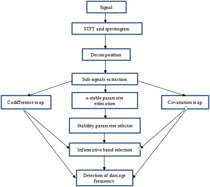
The scheme of the proposed algorithm based on the $\alpha$-stable distribution approach we present in Fig. 1.

Fig. 1Flow chart of proposed procedure

3. Simulated data analysis

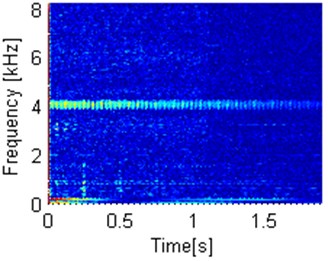
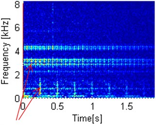
In this section we present simulated time series analysis, see Fig. 2. The investigated signal acquisition parameters are as follows, frequency sampling 16384 Hz and 2.5 s length of the signal. Fig. 3 shows spectrogram of the signal with Kaiser window of length 500, number of overlapping samples being 475, number of samples used for FFT equal to 512, and frequency sampling as was mentioned. It can be seen that there exists cyclic damage. Moreover there is also visible single impulse (artifact). Observing spectrogram, it reveals IFB around 4 kHz, high energy – low frequency band and low energy – high frequency band.

In order to select the informative frequency band we can construct the maps based on the autocovariation and autocodifference, the main measures of dependence adequate for models based on the α-stable distribution. Fig. 4 contains autocodifference and autocovariation maps for sub-signals related to appropriate frequencies from the spectrogram.

As we observe, in linear scale, there is no visible pattern in autocodifference map, however autocovariation map reveals clearly observable IFB. In logarithmic scale, both autocodifference and autocovariation maps allow to identify IFB however autocovariation has superiority over autocodifference map because of removed high energy located in low frequency bands. Both maps successfully remove artifact from original spectrogram.

Fig. 2Raw signal

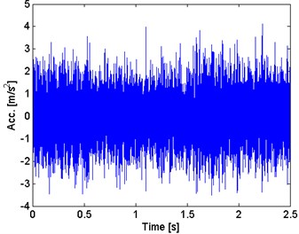
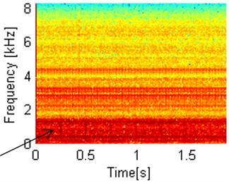
Fig. 3Spectrogram of simulated signal

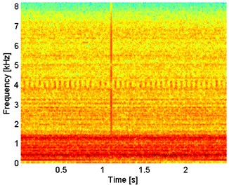
Fig. 4Autocodifference and autocovariation maps in linear and log scale

a) Autocodifference map – linear scale

b) Autocovariation map – linear scale

c) Autocodifference map – log scale

d) Autocovariation map – log scale

As it was mentioned, on the basis of the $\alpha$-stable distribution approach we can also consider the statistic for IFB selection, which is defined in Eq. (6). In Fig. 5 we present a comparison of frequently used selector for informative band, namely spectral kurtosis, and the novel selector based on stability index $\alpha$. As we observe, the $\alpha$-based selector precisely detects informative frequency band, whereas kurtosis is sensitive to single impulse and points wide range frequencies as informative frequency band.

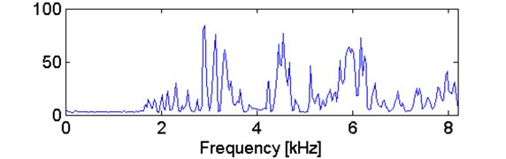
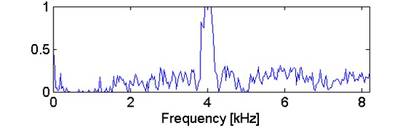
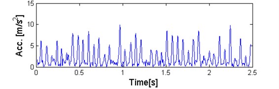
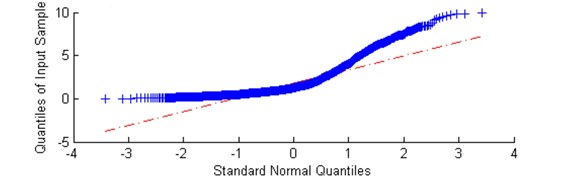
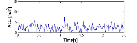
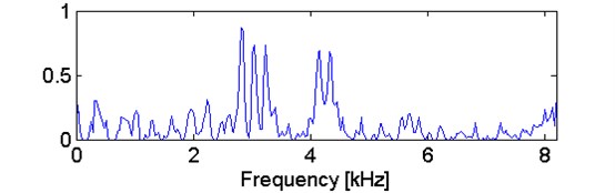
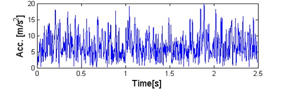
From theoretical point of view, in spectral kurtosis based approach, the kurtosis can be considered as a measure of similarity between empirical distribution of given sample and Gaussian one. If kurtosis value is close to 3, it means that empirical distribution is close to Gaussian one. However, if kurtosis value differ from 3 than consequently hypothesis of Gaussian distribution cannot be accepted. Theoretical kurtosis doesn’t exist for heavy tailed distribution (i.e. for impulsive signals) then in this case it should not be considered. Using an $\alpha$-stable distribution approach provides more elegant and theoretically consistent solution. If given sub-signal contains impulses, it means that distribution might have heavy tails and consequently might be modelled using $\alpha$-stable distribution with $\alpha$-parameter smaller than 2. On the other hand, if given sub-signal doesn’t contain impulses, the signal can be modelled by $\alpha$-stable distribution with $\alpha$-close to 2 that practically means Gaussian. In order to prove that $\alpha$-stable distribution is more appropriate to the considered signal in comparison to the Gaussian distribution approach, in Figs. 6 and 7 we present the exemplary time series corresponding to two frequency bins, namely 4 kHz, with maximum value of novel selector and lies within informative frequency band (Fig. 6) and 4.3 kHz with minimal value of selector, lying outside IFB (Fig. 7).

Fig. 5a) Comparison of kurtosis and b) stability parameter for simulated signal

a)

b)

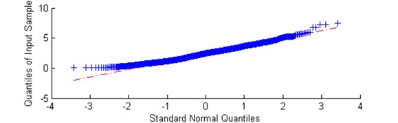
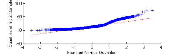
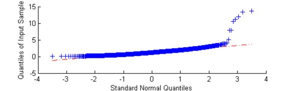
Fig. 6a) Plot of sub-signal corresponding to f= 4 kHz with high value of the α-based selector and b) QQ plot vs. Gaussian distribution

a)

b)

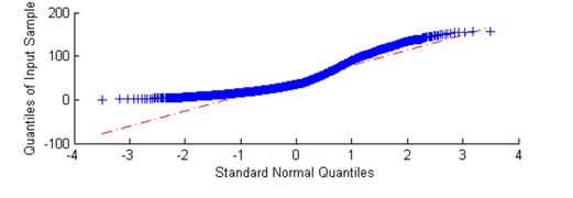
For all of them we apply the classical visual test for Gaussianity, namely the quantile-quantile plot (QQ plot) on which the empirical quantiles and theoretical ones (from Gaussian distribution) are compared. If the examined data set constitutes sample from Gaussian distribution, then the empirical quantiles (blue stars) lie exactly on the theoretical counterparts (red dashed line). Comparing QQ plots placed below it can be clearly seen that in case of high value of selector (Fig. 6) quantiles deviate strongly from theoretical quantiles of Gaussian distribution. It means data are highly impulsive and heavy tailed. In case of low value of selector (Fig. 7), quantiles are more aligned according to the theoretical values corresponding to Gaussian distribution. As a summary, taking into account the fact that for $\alpha =$ 2 the $\alpha$-stable distribution reduces to Gaussian and the fact that for time series related to IFB the distribution is more heavy tailed that in the Gaussian case we can conclude the $\alpha$-stable distribution corresponds to empirical distributions of sub-signals taken from the spectrogram and therefore the proposed approach seems to be more adequate to considered signal.

Fig. 7a) Plot of sub-signal corresponding to f= 4.3 kHz with low value of the α-based selector and b) QQ plot vs. Gaussian distribution

a)

b)

4. Real data analysis

In this section we present basic information about machine, experimental setup and obtained real vibration signal from two-stage, high-power gearbox used in mining industry.

4.1. Machine description and experimental setup

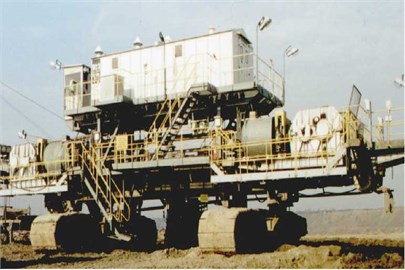
The proposed methodology was developed to condition monitoring of heavy duty machines used in mining industry. Mining machines seem to be a special class of machines with complex structure, high-power, time-varying load etc. In this paper, we will concentrate on a belt conveyor system, widely used for continuous transport of bulk materials (coal, overburden, copper ore, etc.) in both opencast and underground mines. Depending on the design (required power for driving on belt conveyor driving station (Fig. 8) might consist of one up to four drive units with 630 or 1000 kW power each. In our research 630 kW two stage gearbox was considered.

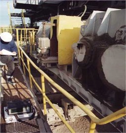
Vibration signals were registered by Bruel&Kjaer Pulse System. About a dozen measurement sessions were carried out in different load conditions and time periods. The registered fragments lasted 2.5 s or 5 s and the sampling frequency was 8192 Hz (or 2×8192 Hz). Several channels were acquired. Locations of accelerometers are presented in Fig. 9. In this paper we use vibration signal acquired from channel 4, an accelerometer placed horizontally on the machine housing.

In Fig. 9 a kinematic scheme of analysed gearbox is presented. It is a two stage gearbox, first stage is a bevel one with helical gears while second one is cylindrical with spur gears. Numbers of teeth on gears are: $z_1=$ 23, $z_2=$93, $z_3=$36, $z_4=$113. Rotation speed of the drive is equal to $n_1=$980 RPM (might vary in time due to varying load). Table 1 contains basic diagnostic parameters of the gearbox, i.e. mesh frequencies and shaft frequencies.

Fig. 8a) Mechanical system used to validate proposed techniques and b) location of sensors on the gearbox housing

a)

b)

Fig. 9Location of sensors – scheme

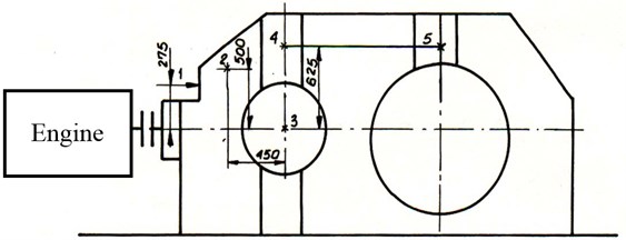
Fig. 10Kinematic scheme of two-stage gearbox. zi denote gears, where ni denote number of RPM’s

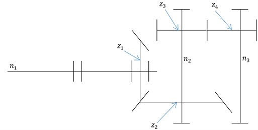
Table 1Basic frequencies of the kinematic scheme

Component name	Frequency [Hz]	Value [Hz]
$f_{01}$ first shaft frequency [Hz];	$f_{01}=n_1/60$	16,52
$f_{02}$ second shaft frequency [Hz];	$f_{02}=n_2/60=n_1/(60\bullet u_1)$	4,06
$f_{03}$ third shaft frequency (output) [Hz];	$f_{03}=n_3/60=n_1/(60\bullet u_1\bullet u_2)$	1,29
$f_{z1}$ first stage mesh frequency [Hz];	$f_z=n_1\bullet z_1/60$	382
$f_{z1}$ second stage mesh frequency [Hz];	$f_z=n_2\bullet z_2/60$	148
$n_1$ rotational speed of first shaft (input) [rpm]; $n_2$, $n_3$ rotational speed of: second and third shaft[rpm]; $u_1$, $u_2$ gear ratio: I stage and II stage gear; $z_1$ number of teeth of first gear; $z_2$ number of teeth of second gear.

4.2. Vibration data selected for analysis

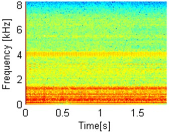
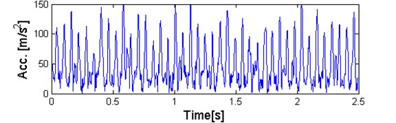
As an example of real data we consider a raw vibration signal of a two-stage gearbox that operates in open-pit mine (Fig. 11) under regular load. Based on preliminary analysis of the signal it is supposed that the gearbox indicates two types of damage. They are related to: distributed damage for second shaft and local damage for first shaft (4.1 Hz and 16.5 Hz, respectively). First problem can be easily noticed even from raw vibration series, Fig. 11.

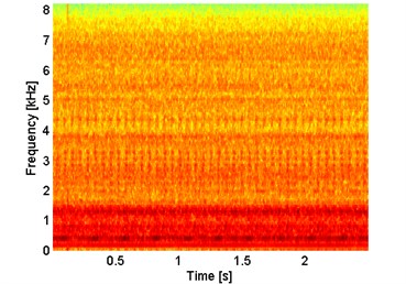
In Fig. 12 we present spectrogram of raw vibration signal with three types of bands: the first one, low-frequency, high-magnitude responsible for shape of the signal while the second and third which are related to informative bands about damage, placed between 2-3.5 kHz and 4-5 kHz. Due to operation of machine, it was not possible to confirm presence of damage by visual inspection. However, properties of the signal (impulsiveness and cycle related to the shaft frequency) clearly indicate fault. Another interesting feature is artifact, probably from random hit on the gearbox during acquisition of signal.

Fig. 11Raw signal from two-stage gearbox

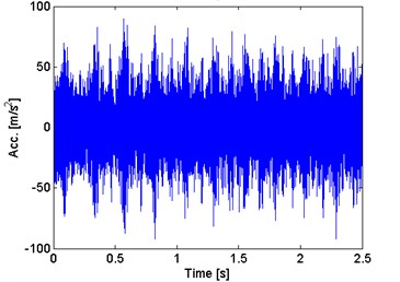
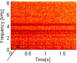
Fig. 12Spectrogram of signal from damaged two-stage gearbox

4.3. Application of proposed method

In this section we will analyse result of application of proposed method in section 2. Signal presented in Fig. 11 has been transformed to time-frequency spectrogram (Fig. 12). Next, Codifference and covariation as well as $\alpha$-stable distribution parameters have been estimated for each spectrogram slice (sub-signal take for each frequency bin).

By using the $\alpha$-stable distribution approach first we observe the maps based on the autocovariation and autocodifference, measures of dependence described in the previous section. In Fig. 13 there are presented mentioned dependency maps for sub-signals taken from the spectrogram. It can be observed that autocovariation map is more sensitive towards the damage.

In linear scale as well as in the log scale we clearly observe two damages. One repeating on the multiples of 0.245 s which relates to 4.0816 Hz frequency of damage of the locally damaged second shaft and second one repeating on the multiples of 0.06 s, which closely relates to the distributed damage of the first shaft frequency, meaning 16.6 Hz. Autocodifference map in linear scale detects only damage from the first shaft. In log scale, second damage also can be detected, but it is significantly more difficult to achieve in comparison to autocovariation maps. Flaw of great significance is autocodifference’s sensitivity to energy contained in spectrogram sub-signals.

In Fig. 14 where we compare the spectral kurtosis and the new statistic defined in Eq. (6), one can clearly see that stability parameter selector is in a large degree insensitive to artifacts contained in the signal in contrast to kurtosis. It can be noticed, that informative frequency bands are detected at ease with novel selector, whereas kurtosis cannot detect them and is highly sensitive to artifact.

Similar as for the previous analyzed signal, also in this case we analyze the exemplary sub-signals taken from the spectrogram, see Figs. 15-18 and comparison of their empirical distribution and Gaussian distribution by using QQ plots, see Figs. 15-18.

Fig. 13Codifference and covariation maps in linear scale and log scale. Arrows indicate fault location on dependency maps

a) Autocodifference map – linear scale

b) Autocovariation map – linear scale

c) Autocodifference map – log scale

d) Autocovariation map – log scale

Fig. 14a) Comparison of kurtosis and b) stability parameter selector for two-stage gearbox signal

a)

b)

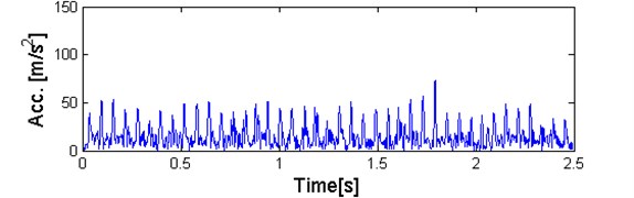
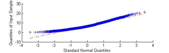
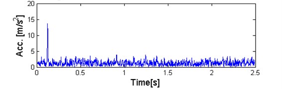
Observing Figs. 15-18 one can easily deduce that for data coming from informative bands with high value of the $\alpha$-based selector QQ plots deviate in tails from standard Gaussian distribution, and plots of sub-signals is ‘spiky’ with impulses coming from damage, where for data from non-informative bands with low value of the selector data are less impulsive and quantile-quantile plots are highly aligned with theoretical quantiles of Gaussian distribution. One exception is sub-signal from band where artifact is clearly observable. For sub-signal with one spike (Fig. 18), related to artifact, quantile-quantile plot is highly aligned with theoretical values of Gaussian distribution, with few outliers connected with aforementioned artifact. Summarizing real signal analysis, the approach based on the $\alpha$-stable distribution seems to be more adequate in the contrast to the classical Gaussian approach.

Fig. 15a) Plot of sub-signal corresponding to f= 2,8 kHz with high value of the α-based selector and b) QQ plot vs. Gaussian distribution

a)

b)

Fig. 16a) Plot of sub-signal corresponding to f= 4,1 kHz with high value the α-based selector and b) QQ plot vs. Gaussian distribution

a)

b)

5. Conclusion

In the paper a novel criteria for local damage detection are proposed. The approach is based on the fundamental property of a vibration signal from a damaged machine, i.e. presence of impulses in a certain frequency band. As an indicator of impulsiveness we used the stability parameter of the $\alpha$-stable distribution which is frequently used to description of impulsive signals. The choice of this parameter is motivated by the fact that it is close to a certain constant for a sub-signals that represent healthy machine or the non-informative part of the signal from a damaged machine while stability parameter is significantly lower for frequency bands containing impulses, i.e. from informative frequency bands. Additionally, novel time-frequency maps are proposed here. The maps are constructed on the basis of the measures of dependence appropriate for $\alpha$-stable distribution, since in case of data being heavy-tailed, theoretical values of autocorrelation are infinite. Using novel time-frequency maps together with $\alpha$-based selector, provides suitable tool for detection of damage, with high degree of insensitivity towards artifacts and random errors in acquisition of data. Furthermore, using these method allows us to detect multiple damages with high precision, which was confirmed in experimental setup.

Fig. 17a) Plot of sub-signal corresponding to f= 7,3 kHz with low value of the α-based selector and b) QQ plot vs. Gaussian distribution

a)

b)

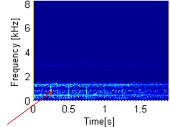
Fig. 18a) Plot of sub-signal corresponding to f= 7,9 kHz with low value of the α-based selector and high value of kurtosis and b) QQ plot vs. Gaussian distribution

a)

b)