Sectional normalization and recognization on the PV-Diagram of reciprocating compressor

1. Introduction

Reciprocating compressors are widely used in petroleum, chemical, transportation and other industrial fields. The statistical analysis shows that the high fault probability is present in the cylinder subassembly of reciprocating compressor. The result is that the reciprocating compressor is shut down in order to examine and repair, and the economic benefit of enterprise is affected badly. The PV-Diagram of the reciprocating compressor can reflect the change course of gas pressure in the cylinder during a gas compression cycle. It is a true record of operating state about the cylinder [1]. The PV-Diagram with the fault characteristics is formed when there are faults in the cylinder subassembly. An accurate diagnosis about the faults of the cylinder subassembly can be made by identifying the PV-Diagrams with different characteristics. For the state monitoring and fault diagnosis of reciprocating compressor, the most effective method is measuring directly the dynamic pressure in the cylinder, and drawing the PV-Diagram or the pressure change curve, and identifying the faults of compressor by comparing with the pressure change curve of normal operating condition.

The PV-Diagram’s contour and shape are the first important for identifying the faults of compressor, and its actual size and location are secondary. The measured PV-Diagram under different conditions must be normalized for the automatic recognizing. After the PV-Diagram is normalized, its original shape characteristics must be maintained, and the running state information of compressor must be reserved. And the normalization method can facilitate analyzing and processing for the PV-Diagram with computer. In this paper, a sectional normalization method of the PV-Diagram of reciprocating compressor was put forward base on analyzing the shortcomings of familiar normalization method.

The structural risk minimization principle is adopted in Support Vector Machines (SVMs), and training error and generalization capabilities are taken into account. Therefore SVMs has unique advantages in processing small-sample data sets and non-linear problems, and it is particularly suitable for establishing a multi-fault classifier [2]. In this paper, a multi-fault classifier was established with SVMs in order to recognize the typical fault PV-Diagrams of reciprocating compressor that have been normalized.

2. Sectional normalization method of the PV-Diagram

The study object is 2D12-70/0.1~13 opposed double action gas compressor. The main parameters are as follows: shaft power is 500 kW, displacement is 70 m³/min, exhaust pressure of grade I is 0.2746-0.2942 MPa, exhaust pressure of Grade II is 1.2749 MPa, piston stroke is 240 mm, crankshaft rotating speed is 496 r/min. 2D12 compressor is double-acting compressor that has two cylinders. In order to detect the pressure change of each working chamber, each compressor should be equipped with four sets of pressure measurement devices [1]. There are four exhaust valves and four intake valves on each working chamber of grade I cylinder. There are two exhaust valves and two intake valves on each working chamber of grade II cylinder. All these valves are ring valve featuring multiloop narrow channels and low stroke. The intake valves are on the top of the cylinder, and the exhaust valves are on the bottom of cylinder.

A PV-Diagram of cap side of the grade II cylinder under normal operating condition is shown in Fig. 1. A gas compression cycle can be divided into four stages: expansion, suction, compression and exhaust. The upper dead centre signal of piston motion is given by a keyphase sensor. The upper dead centre is defined as a starting point of the expansion stage (c), the pressure minimum point as a starting point of suction stage (d), the bottom dead center as a starting point of compression stage (a), the pressure maximum point as a starting point of exhaust stage (b). A gas compression cycle curve is divided by these four points as expansion stage (c-d), suction stage (d-a), compression stage (a-b), and exhaust stage (b-c). By analyzing the impact of different faults on the PV-Diagram can be found that the effect of different faults on the four stages is different. The curve of expansion stage will shift to the right when the exhaust valve leak happens, and the curve of compression stage will shift to the left when the intake valve leak happens. Thus, the relative shape difference between fault PV-Diagram and normal PV-Diagram should be kept after normalization, or an accurate fault diagnosis can’t be made for the compressor.

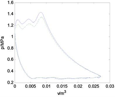
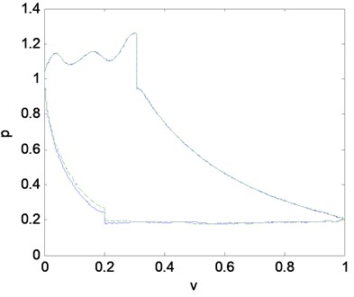
There are two familiar methods for normalization. First method is that the minimum and maximum pressure of PV-Diagram is defined as 0 and 1, second is that the gas entry pressure (the pressure of the upper dead centre, $p_d$) and exhaust vent pressure (the pressure of the bottom dead center, $p_s$) of the cylinder is defined as 0 and 1. The contrast between the normal PV-Diagram and the fault PV-Diagram that was brought with a decrease in spring stiffness is shown in Fig. 2. The PV-Diagram after normalization with the first method is shown in Fig. 3. The maximum pressure was transformed into 1, and the relative shape of the normal and the fault PV-Diagram was changed. As a result, the phenomenon that the opening pressure of exhaust valve has fallen can’t be showed intuitively when the spring stiffness is diminished. In these figures of this paper, the solid line indicates the normal PV-Diagram, the dotted line indicates the fault PV-Diagram, the abscissa represents volume, the ordinate represents pressure, and both parameters are dimensionless. The second method results in the change of the relative shape of PV-Diagram also. Fig. 4 shows the actual comparison PV-Diagrams of normal state and intake valve leakage on cap side of the grade II cylinder. Fig. 5 shows the comparison PV-Diagrams that are normalized with the second method. We can see that the curvatures of expansion stage line and compression stage line have changed in comparison with Fig. 4, and the shift left feature of the compression stage line in fault condition has changed to the shift right.

According to thermodynamic theory, isothermal equation is $Pv=C_1$, isentropic equation is $P{v}^k=C_2$, polytrope equation is $P{v}^m=C_3$. Where $p$ is pressure, $v$ is specific volume, $k$ is isentropic index, $m$ is polytrope index, and $C_1$, $C_2$ and $C_3$ are constant. Besides the nature of gas, the polytrope index primarily depends on the heat interchange between gas and external world, and the energy loss in the gas flow process. Under normal conditions, the temperature of the cylinder and the piston is always higher than the intake temperature after the compressor works for a period of time. So that the gas is heated by the cylinder and the piston in the intake process, and the gas temperature has gone up. In the exhaust stage, the gas temperature is higher than the cylinder wall’s, so the gas gives off heat and the gas temperature has come down. The heat exchange state is very complicated in compression and expansion process. Sometimes the gas gives off heat to the cylinder, and sometimes absorbs heat from the cylinder. For example, the gas temperature is lower than the temperature of cylinder wall in the front part of the compression stage (a-b), so the gas absorbs heat. If you use the polytrope equation to represent the heat exchange state, $m$ should be greater than $k$ in the equation. The compression stage is continuing until the gas temperature and cylinder wall temperatures are equal, $m$ should be equal to $k$ at this time. The gas temperature is higher than the temperature of cylinder wall in the late part of the compression stage, so the gas gives off heat, and then $m$ is less than $k$. For the expansion stage (c-d), the gas gives off heat in the front part, $m>k$, the gas absorbs heat in the late part, $m<k$. Therefore, the lines of the expansion stage or the compression stage can’t be expressed by an exponential function in which the index $m$ is a constant. If the model were used, the index of the equation should be a variable. Although the reciprocating compressor is water-cooled or air-cooled commonly, generally $1<m<k$, $m$ is always changing in a gas compression cycle of compressor.

Fig. 1The normal condition PV-Diagram of reciprocating compressor that works in actual state

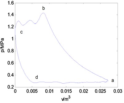
Fig. 2Comparison PV-Diagrams between fault condition of exhaust valve spring and normal condition that measured in actual state

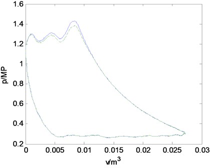
Fig. 3Comparison PV-Diagrams between fault condition of exhaust valve spring and normal condition after normalization with the first method

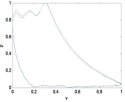
Fig. 4Comparison PV-Diagrams between intake valve leakage condition and normal condition that measured in actual state

The reason that the familiar normalization method causes the shape of PV-Diagram to change is the curvature of PV-Diagram happens to change, or the mapping relation between pressure and specific volume happens to change. As shown in Fig. 3, the pressure is normalized as follows:

For any two states (1 and 2) of compression stage or expansion stage, the polytrope equation is given by:

After normalized, the polytrope equation is as follows:

Obviously, $m_2\ne m_1$, the shape of PV-Diagram is changed. The same conclusion is given by analyzing the normalization method as shown in Fig. 5, just the shape change of suction stageline and exhaust stage line is relatively smaller.

Fig. 5Comparison PV-Diagrams between intake valve leakage condition and normal condition after normalization with the second method

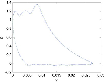
Fig. 6Comparison PV-Diagrams between intake valve leakage condition and normal condition after normalization with the new method

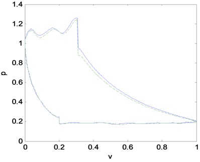
Fig. 7Comparison PV-Diagrams between exhaust valve leakage condition and normal condition that measured in actual state

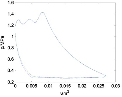
Fig. 8Comparison PV-Diagrams between exhaust valve leakage condition and normal condition after normalization with the new method

Based on the above analysis, we can’t use the simplified method in the course of the PV-Diagram normalization. A new method was put forward in this paper. First, the PV-Diagram has been normalized in the volume direction. Then, the PV-Diagram will be normalized separately after it is divided into two parts. The first part is composed of the expansion stage line and the exhaust stage line. The real pressure of the part will be divided by the pressure of the upper dead centre ($p_d$). The second part is composed of the compression stage line and the suction stage line. The real pressure of the part will be divided by the pressure of the bottom dead center ($p_s$), and then multiplied by a coefficient $c$. The function of $c$ is favorable to the reconstructed PV-Diagram expresses the shape of the real PV-Diagram better. We use $n_1$ to indicate the breakpoint between the expansion stage line and the suction stage line, and $n_2$ to indicate the breakpoint between the compression stage line and exhaust stage line. The value of $n_1$ and $n_2$ depend on the structural and thermal character of the compressor, and commonly should be taken before the minimum pressure point and the maximum pressure point. Fig. 4 shows a real PV-Diagram. After Fig. 4 has been normalized with the new method, the PV-Diagram is shown in Fig. 6. Relative to the original figure, the curvature of four sections of curve that indicate four stages of a gas compression cycle has not changed after the PV-Diagram is normalized, and keeps the interrelations of contour and shape between normal and fault state characteristic curve. Fig. 7 shows the actual comparison PV-Diagrams between normal and exhaust valve leakage state. Fig. 8 shows the comparison after the PV-Diagrams are normalized sectionally and reconstructed. The superiority of the new method has been further verified.

3. Multi-fault classifier based on support vector machine

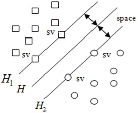
Support vector machine (SVM) theory [3] is put forward for two-class pattern recognition problem, and its basic idea can be illuminated by a two-dimensional system as shown in Fig. 9. The circles and the squares in the diagram represent the two classes of samples. $H$ is a classification line. $H_1$ and $H_2$ pass through the samples which are nearest to the classification line among all the samples, and these two straight lines are parallel to the classification line. The samples on the $H_1$ and $H_2$ are called support vectors. The distance between $H_1$ or $H_2$ and $H$ is called classification space. It is the so-called optimal classification line that is able not only to separate the samples into two classes correctly (error rate of training is 0), but also to achieve the maximum of classification space. The nonlinear problems can be translated into linear problems of high-dimensional space through nonlinear transformation, and the optimal classification surface can be obtained in transformation space.

Fig. 9The optimal classification line in a two-dimensional system

SVM is a learning machine which is designed for dual classification problem, and it can not be used directly to solve multiple classification problems. But, a multiple classifier is needed for identifying the PV-Diagrams, in other words, an effective method is needed to extend the SVM from dual classifier to multiple classifier.

Many scholars have studied this issue and put forward some effective methods. These methods can be divided into two types. One type is that a multiple classifier is composed of many dual classifiers. Take, for example, the one-against-all multi-classification algorithm. For classification problem with $K$ classes, this algorithm needs to construct $K$ SVMs. The training sample of $i$-th SVM is produced by the method that the samples in the $i$-th class are marked for one category, while the samples of all other classes for another category. The class of a new sample depends on the biggest output value of $K$ SVMs. Another main method is one-against-one classification algorithm. Every dual classifier is trained with two classes of $K$ training samples only. In this way, $K(K-1)/2$ dual classifiers can be built all together. In the classification process, we can adopt the voting method. That is to say, after a data is inputted some classifier, we can acquire a classification result. If this result belongs to $m$-th class, the $m$-th class is added a vote. After the data is classified by all classifiers, then the data belongs to the class which gets the most votes.

For the fault diagnosis problem of mechanical equipment, the fault class number $K$ is generally between 5 and 15. Because the fault probability of mechanical equipment is very low, the fault sample number $n$ is fewer normally. Based on these characteristics, in this paper, we use the one-against-all multi-classification algorithm to construct the multi-fault classifier.

4. Identifying of the PV-Diagram

On the basis of analyzing the common fault of cylinder subassembly on 2D12 compressor, we have done many simulation experiments on the compressor set of a compression gas station. A large amount of data has been collected. The PV-Diagrams under five operating modes have been obtained. The five modes are respectively normal operating condition, intake valve leakage condition, exhaust valve leakage condition, cylinder clearance fault condition and cylinder piston fault condition. Among them, the intake valve leakage condition leads to the result that the curve of compression stage on PV-Diagram shifts to the left, as illustrated in Fig. 6. The exhaust valve leakage condition leads to the result that the curve of expansion stage on PV-Diagram shifts to the right, as illustrated in Fig. 8. The training sample set is constructed with pressure signals which are collected in the simulation experiments. 500 pressure signals are extracted from the datum of every operating mode. PV-Diagram of every sample is normalized sectionally and reconstructed. 120 uniformly-spaced points are extracted on the curve of PV-Diagram and used as feature vectors of every operating mode. If feature points were extracted too many, it would increase the workload of training and recognition on fault diagnosis model. However, if feature points were extracted too few, it would be insufficient to reflect the state characteristic of PV-Diagram. After comprehensive consideration, we form a feature vector from 120 feature points.

For the Support vector machine, parameters of kernel function and error punish parameter $C$ are the main factors that affect its performance. Actually, the variation of parameters of kernel function will change implicitly the mapping function, and thus leads to the change of the sample distribution complexity in the data subspace (dimension). In the determinate data subspace，the function of the error punish parameter $C$ is regulating the confidence range of learning machine and the ratio of empirical risk on the risk boundary. After $C$ has been given, the level of empirical risk on the risk boundary is also determined. Then we can gain the simplest optimal classification surface on which the given level of empirical risk is achieved through solving support vector machines. Optimizing the parameters of support vector machines is the precondition to ensure that it has excellent generalization capability.

In this paper, polynomial is chose as kernel function of support vector machines. The parameter of kernel function that is required to set up is the order of polynomial. In the training process, in addition to 500 pressure signals are chosen as the training sample set, 300 pressure signals are chosen for the testing sample set. We use cross-validation method to determine the optimal parameters [4]. For the polynomial support vector machine, the parameter set of polynomial order $q$ and error punish parameter $C$ is first required to construct. The parameters of set are chosen and combined, and then used in the training of support vector machines. Secondly, the support vector machines are tested with the testing sample set, and the optimal parameter combination is chosen according to the error rate of recognition. The testing result is that $q$ is 4, and $C$ is 100.

In order to test the superiority of the sectional normalization method of PV-Diagram, the same training samples and testing samples are normalized with different normalization methods and used to construct the training sample sets and the testing sample sets respectively, the same structure classifier based on support vector machine is trained and tested with these different sets. The result shows that the recognition correction rate of classifier for compressor faults can be significantly improved with the sectional normalization method of PV-Diagram.

5. Conclusion

After a PV-Diagram is normalized with the familiar normalization methods, the curvature of curve on the PV-Diagram is changed. The PV-Diagram’s relative contour and shape are also changed in varying degrees. Of course, the automatic recognition of the PV-Diagrams under different operating modes is also difficult to realize. On the basis of the analysis on the transformation regularity of the PV-Diagram, a sectional normalization method of the PV-Diagram was put forward in this paper. After a PV-Diagram is normalized with the new method, the curvature of four sections of curve that indicate four stages of a gas compression cycle are unchanged in comparison with the original diagram. The relations between the feature curves of normal and fault operating modes on the contour and shape are retained.

Through simulating experiments for five operating modes, a large amount of data for cylinder piston system of the compressor was collected. After the PV-Diagrams were processed with different normalization methods, and used in the training and testing for the same structure support vector machines. The result indicated that sectional normalization method has obvious superiority.

References

-
Wang J. D., Zhang J. Z., Yang J. Y. Technique to detect the gas pressure in cylinder of 2D12 reciprocating compressor. Compressor Technology, Vol. 5, 2002, p. 21-23.
Zhang Z. S., Li L. J., He Z. J. Multi-fault classifier based on support vector machine and its applications. Mechanical Science and Technology, Vol. 23, Issue 5, 2004, p. 536-537.
Cortes C., Vapnik V. Support vector networks. Machine Learning, Vol. 20, 1995, p. 273-397.
Jiang A. N., Feng X. T. Case-based SVM method for maximal deformation forecasting of surrounding rocks of tunnels. Journal of Northeastern University (Natural Science), Vol. 25, 2004, p. 793-795.
About this article