Abstract
A novel approach on kernel matrix construction for support vector machine (SVM) is proposed to detect rolling element bearing fault efficiently. First, multi-scale coefficient matrix is achieved by processing vibration sample signal with continuous wavelet transform (CWT). Next, singular value decomposition (SVD) is applied to calculate eigenvector from wavelet coefficient matrix as sample signal feature vector. Two kernel matrices i.e. training kernel and predicting kernel, are then constructed in a novel way, which can reveal intrinsic similarity among samples and make it feasible to solve nonlinear classification problems in a high dimensional feature space. To validate its diagnosis performance, kernel matrix construction based SVM (KMCSVM) classifier is compared with three SVM classifiers i.e. classification tree kernel based SVM (CTKSVM), linear kernel based SVM (L-SVM) and radial basis function based SVM (RBFSVM), to identify different locations and severities of bearing fault. The experimental results indicate that KMCSVM has better classification capability than other methods.
1. Introduction
Rolling element bearing (REB) is a critical unit in rotating machinery and its health condition is often monitored to identify incipient fault. When a defect like bump, dent or crack that occurs in REB' outer race, inner race, roller or cage, continuously contacts another part of bearing under operation, a sequence of impulsive responses can be acquired in the form of vibration [1-3], acoustic emission [4], temperature, motor current, ultrasound [5], etc. However, the measured signals involve both fault-induced component and noises from structure vibration, environment interference, etc. Furthermore, fault-induced signal is often masked by noises due to its relatively low energy. In fact, many signal processing techniques including time domain analysis, frequency analysis and time-frequency analysis have been explored to draw fault signatures effectively. For example, Statistical parameters in time domain are used as defective features such as RMS, Variance, Skewness, Kurtosis, etc. [6, 7]. Features are derived from time series model like the Autoregressive [8, 9]. Frequency analysis aims to find whether characteristic defect frequency (CDF) exists in spectrum [10-14]. As non-stationary signals, bearing fault signals are extensively dealt with using time-frequency analysis to obtain local characteristic information both in time and frequency domain [15-17]. Two or more kinds of signal processing techniques are also combined together for feature extraction [18-20]. Some signal analysis methods have been optimized before performing feature extraction [21, 22] like flexible analytic wavelet transform [23] by employing fractional and arbitrary scaling and translation factors to match fault component. High-dimension features could be compressed into low-dimension features by optimal algorithms [24-26] like manifold learning [27-30] for efficient diagnosis. Due to its complexity of bearing, it is almost impossible for even domain experts to judge the bearing condition just by inspecting the characteristic indices. In order to automate diagnosis procedures and decision-making on REB health state, a variety of automatic diagnosis methods have been put forward such as artificial neural network (ANN), support vector machine (SVM), fuzzy logic, hidden Markov model (HMM) and other novel approaches [31]. In [32], the anomaly detection (AD) learning technique has got higher accuracy than SVM classifier for bearing fault diagnosis. The trifold hybrid classification (THC) approach can isolate unexampled health state from exampled health state and discriminate them exactly [33]. Simplified fuzzy adaptive resonance theory map (SFAM) neural network is investigated and able to predict REB remaining life [34]. A poly-coherent composite spectrum (PCCS), retaining amplitude and phase information, is observed to have a better diagnosis than methods without phase information [35]. HOS-SVM model, which integrates high order spectra (HOS) features and SVM classifier, indicates the capability of diagnosing REB failures [36].
As mentioned above, great progress has been made in detecting bearing conditions. Meanwhile, these proposed methods also face some challenges. For instance, owing to the fluctuation in speed or load, a measured CDF is probably inconsistent with the theoretical calculation. The selection of base wavelet and scale levels mostly relies on researchers’ experience and prejudice rather than objective criterions. The discrete wavelet transforms (DWT) still suffers from limitations of fixed scale resolution regardless of signal characteristics. The structures of ANN, particularly initial weights, which are randomly determined by trial and experience, may weaken generalization capability and training velocity. For SVM classifier, the kernel function is demanded to map samples from an input space to a higher feature space where the samples can be linearly separated. However, the kernel function confines to typical formulas such as linear, polynomial, radial, multilayer perception and sigmoid function which will not surely succeed in search of the intrinsic correlation among the samples. Consequently, it possibly contributes to poor classification.
Thereby, a novel method on kernel matrix construction for SVM (KMCSVM) is proposed to identify REB fault more precisely. Two kernel matrices, i.e. the training kernel matrix and the prediction kernel matrix , are constructed in this way. The matrix exposes the similarity of intrinsic characteristics among training samples, while the matrix specifies the similarity between training samples and test samples. The results show that KMCSVM has better ability for REB fault diagnosis. To our best knowledge, KMCSVM has not been observed in rotating machinery fault diagnosis fields.
The rest of this paper is organized as follows: Section 2 reviews the background knowledge about CWT and singular value decomposition (SVD) for feature extraction. The procedure based on KMCSVM is presented in Section 3. The proposed method is validated by identifying bearing fault locations and severities in Section 4. Finally, conclusions are drawn in Section 5.
2. Methods review
Because signals from defective bearing are non-stationary, nonlinear, local and transient, CWT is chosen to process the signals and SVD is used to calculate the eigenvector from the coefficient matrix as signal signature.
2.1. Continuous wavelet transform
CWT aims to measure a local similarity between wavelet at scale position and signal . The wavelet coefficient can be defined by Eq. (1):
By shifting in time and scaling , a wavelet coefficient matrix can be created which is viewed as a time-frequency space as Eq. (2) and represents the dynamic characteristics of the signal :
where is the coefficient at the th scale and at the th data point of a sample signal.
2.2. Singular value decomposition
SVD is used to decompose the wavelet coefficient matrix . Assuming matrix with the size of , the SVD results can be expressed by Eq. (3):
where and are orthogonal matrices of and , respectively. is an diagonal nonnegative matrix. The diagonal elements in are called singular values (SVs) of , which are only determined by matrix itself and denote the natures of matrix , namely, the characteristics of a sample signal. Given , Eq. (3) can be illustrated in details as Eq. (4):
SVs constitute vector described as Eq. (5). also denotes the feature vector extracted from a sample signal:
3. Proposed method
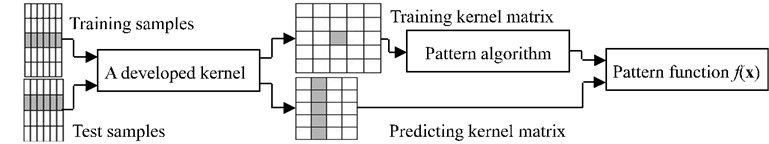
SVM is well suited for linear pattern recognition. However, the original feature vectors extracted from REB are not linearly separated. Suppose there exists a high dimensional space where the original feature vectors are mapped into the high dimension feature vectors that can be linearly separated using SVM in it, the linear pattern recognition based SVM turns to find kernel matrices with the inner product between the imaged high dimension feature vectors. Fig. 1 shows the stages of kernel pattern analysis. The sample feature vectors are used to create training and predicting kernel matrix. The pattern function then uses the matrices to recognize unseen samples. For kernel pattern analysis, the key is how to construct kernel matrices.
Fig. 1Stages in the implementation of kernel pattern analysis
3.1. Kernel matrix pattern based SVM
A training set and a test set are given as below:
Assume is a image of point mapped into a high dimensional feature space and all the sample images can be separated by a hyper-plane as Eq. (8):
The hyper-plane is determined to solve the following optimization problem:
It is equivalent to solving a constrained convex quadratic programming optimization problem:
is named training kernel matrix which is a symmetric matrix with , the inner product between the images of two training samples in space . is the number of training samples, is a column vector with , is a Lagrange multiplier vector, is an diagonal matrix with , is error penalty constant, is the th sample class label.
By maximizing , the optimized can be obtained. Thus, the optimized can be computed using the following equation:
where is the th column vector of .
Hence, the pattern function of SVM to predict the class of unseen sample can be written as:
and:
is named prediction kernel matrix of with , the inner product between the images of a training sample and a test sample in space . is the number of the test samples, is the th column vector of .
According to Eq. (15), the result of pattern analysis just depends on kernel matrices, so it is feasible for SVM to solve nonlinear classification problems by developing appropriate kernel matrices.
3.2. Kernel matrix construction
A novel method on kernel matrix construction (KMC) is presented to solve nonlinear classification problems using pattern analysis based SVM.
To our best knowledge, this KMC based method has not been studied in the field of machinery fault diagnosis. The specific procedure of KMC is stated below and illustrated in Fig. 2.
Fig. 2Flow chart of training kernel matrix K construction
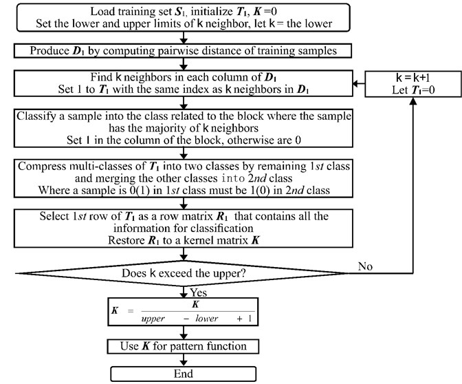
Step 1: Provide training set and test set . Suppose there exists classes of samples in . is used to construct training kernel matrix of . and are used for predicting matrix of . Let be a matrix of , of . Initialize , 0.
Step 2: Produce distance matrix by computing pairwise distance of samples using Eq. (17). Thus, about pairwise distance of training samples and about pairwise distance between training and test samples are shown as Eq. (18):
denotes the distance of the th training sample and the th training sample in and the distance of the th training sample and the th test sample in .
Step 3: Find the closest neighbors distribution of each sample. The closest neighbors of each sample are the least numbers in each column of . Set 1 to the elements in that have the same locations of the least numbers in . The rows of is divided into blocks, its blocks and columns stand for classes and samples, respectively. Eq. (19) shows the k closest neighbors distribution in different classes by setting 1:
Step 4: Classify using majority vote among the neighbors. If a sample has the majority of neighbors within one block, the sample belongs to the block related class. Set 1 to the column within the block, 0 to the rest of that column. For example, if belongs to the 1st class, is revised as Eq. (20):
Step 5: Compress multi-classes of into two classes. The 1st class remains unchangeable and the other classes merge into the 2nd class. Where a sample is 0(1) in the 1st class must be 1(0) in the 2nd class. The updated and are shown as Eq. (21):
Step 6: Select the 1st row of as a row matrix . reveals training samples class, describes test samples class:
The training kernel matrix can be constructed based on , it is an symmetric matrix with diagonal element 1 as Eq. (23). reflects the similarity among training samples. The prediction matrix with can be likewise established according to and . exhibits the similarity between training and test samples. In “1” means the maximum similarity between corresponding samples and “0” means no similarity:
Step 7: Increase and repeat from Step 3 to Step 6 till k exceeds the upper. The upper should be given to a medium value to save computing time.
Step 8: Take the average of the matrices . A number of would be produced with the closest neighbor changing from the lower to the upper. Average these matrices to get better intrinsic relations among samples. The averaged is applied to the pattern function for classification.
4. Case studies
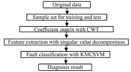
REB fault diagnosis is investigated to validate the effectiveness of KMCSVM. Fig. 3 shows the scheme of REB fault diagnosis.
Fig. 3Flow chart of REB fault diagnosis
4.1. Experimental setup and vibration data
The experiment data about faulty bearings is taken from the Case Western Reserve University Bearing Data Center. The vibration data has been widely utilized as a standard dataset for REB diagnosis. As shown in Fig. 4, the test stand consists of a 2 hp motor (left), a torque transducer/encoder (center), a dynamometer (right), and control electronics. The test bearings support the motor shaft. Motor bearings were seeded with faults using electro-discharge machining. Faults ranging from 0.007 inches in diameter to 0.021 inches in diameter were introduced separately at the inner raceway, rolling element and outer raceway. Faulted bearings were reinstalled into the test motor and vibration data was recorded for motor loads of 0 to 3 horsepower (motor speeds of 1797 to 1720 RPM). Bearing Information is shown as Table 1 and Table 2. Vibration signal was collected using accelerometers, which were attached to the drive end of the motor housing with magnetic bases. Then vibration signal was digitalized through a 16 channel DAT recorder. Digital data was collected at 48.000 samples per second for drive end bearing faults and post processed in a MATLAB environment. Speed and horsepower data were collected using the torque transducer/encoder and were recorded.
Table 1Bearing information: 6205-2RS JEM SKF size: (inches)
Inside diameter | Outside diameter | Thickness | Ball diameter | Pitch diameter |
0.9843 | 2.0472 | 0.5906 | 0.3126 | 1.537 |
In this experiment, the vibration data of the drive end bearing are chosen to perform location and severity identification of bearing fault. The sampling frequency is 48 kHz and each sample contains 2048 data points. Four different bearing conditions, i.e. healthy state, outer race fault, inner race fault and ball fault are observed for fault location recognition using KMCSVM. In addition, four types of fault severities (healthy, 0.007, 0.014 inch and 0.021 inch) are also considered to assess KMCSVM classification performance.
Table 2Fault specifications size: (inches)
Bearing | Fault location | Diameter | Depth | Bearing manufacturer |
Drive end | Inner raceway | 0.007 | 0.011 | SKF |
Drive end | Inner raceway | 0.014 | 0.011 | SKF |
Drive end | Inner raceway | 0.021 | 0.011 | SKF |
Drive end | Outer raceway | 0.007 | 0.011 | SKF |
Drive end | Outer raceway | 0.014 | 0.011 | SKF |
Drive end | Outer raceway | 0.021 | 0.011 | SKF |
Drive end | Ball | 0.007 | 0.011 | SKF |
Drive end | Ball | 0.014 | 0.011 | SKF |
Drive end | Ball | 0.021 | 0.011 | SKF |
4.2. Feature extraction
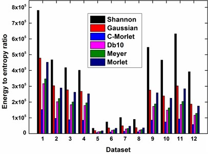
Referring to wavelet selection criterion in subsection “Wavelet selection” presented in [37], the energy to entropy ratios about six different wavelets including the Shannon, Gaussian, Complex Morlet, Daubechies, Meyer and Morlet are plotted in Fig. 5. due to the maximum energy to entropy ratio, the Shannon wavelet is selected as the best mother wavelet to perform continuous wavelet transform. The feature vectors are calculated from the coefficient matrices using SVD.
Fig. 4Rolling element bearing test rig
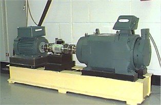
Fig. 5Energy to entropy ratios of datasets using wavelets
4.3. Classification of bearing conditions
The performance of KMCSVM is evaluated by identifying bearing fault location and fault severity, and compared with other kernel pattern recognition methods like CTKSVM, L-SVM and RBFSVM that have been studied in the previous work [37]. CTKSVM is a SVM based on the classification tree kernel which is constructed using fuzzy pruning strategy and tree ensemble learning algorithm to improve the diagnostic capability of REB fault. L-SVM makes use of classical linear kernel as well as RBFSVM with radial basis function to diagnose REB fault. Both five-fold cross validation and independent test are conducted to obtain the classification accuracy of these SVM classifiers. To discover the true fault from the possible multi-faults, SVM classifiers are trained in a tournament of one against others by setting one class as +1 and others as –1, and continuous to detect unknown sample in the same manner.
4.3.1. Identification of fault location
Fault location recognition strives to distinguish four different bearing conditions, i.e. healthy state, outer race fault, inner race fault and ball fault. Table 3 lists 12 datasets with various loading, fault size and shaft speed for analysis. There are 48 samples for each state, thus total 192 samples for all states in each dataset shown as Table 4.
The groups of sample sets are allocated in the way that satisfies the tournament of training and test using five-fold cross validation and independent test as described in Table 5.
Table 3Description of 12 datasets on fault locations
Dataset | 1 | 2 | 3 | 4 | 5 | 6 | 7 | 8 | 9 | 10 | 11 | 12 |
Fault (inch) | 0.007 | 0.007 | 0.007 | 0.007 | 0.014 | 0.014 | 0.014 | 0.014 | 0.021 | 0.021 | 0.021 | 0.021 |
Load (HP) | 0 | 1 | 2 | 3 | 0 | 1 | 2 | 3 | 0 | 1 | 2 | 3 |
Speed (RPM) | 1796 | 1772 | 1750 | 1725 | 1796 | 1772 | 1750 | 1725 | 1796 | 1772 | 1750 | 1725 |
Table 4Composition of dataset on fault locations
Fault type | Sample size |
H | 48 |
O | 48 |
I | 48 |
B | 48 |
H – healthy, O – outer race defect, I – inner race defect, B – ball defect | |
Table 5Sample set with different fault locations for training and test
Sample label | 5-fold cross validation | Independent test | ||
Training | Test | |||
1 | H vs. (O+I+B) | 48: (48 + 48 + 48) | 24: (24 + 24 + 24) | 24: (24 + 24 + 24) |
2 | O vs. (I+B) | 48: (48 + 48) | 24: (24 + 24) | 24: (24 + 24) |
3 | B vs. (O+I) | 48: (48 + 48) | 24: (24 + 24) | 24: (24 + 24) |
4 | I vs. (O+B) | 48: (48 + 48) | 24: (24 + 24) | 24: (24 + 24) |
5 | I vs. B | 48:48 | 24: 24 | 24: 24 |
6 | O vs. I | 48:48 | 24: 24 | 24: 24 |
7 | O vs. B | 48:48 | 24: 24 | 24: 24 |
Fig. 6 illustrates the accuracy of the four classifiers corresponding to the 12 datasets in Table 3 using five-fold cross validation. The classification accuracy of RBFSVM is obviously lowest among all the methods. In eight cases (Fig. 6(b)-(h), Fig. 6(k)), KMCSVM achieves a higher classification accuracy. In three cases (Fig. 6(a), Fig. 6(i), Fig. 6(l)), the classification rates based on KMCSVM, CTKSVM and L-SVM are almost similar to each other. Only in one case (Fig. 6(j)), the classification accuracy of KMCSVM is slightly lower than those of CTKSVM and L-SVM. As a whole, the classification ability increases in the order of RBFSVM, L-SVM, CTKSVM and KMCSVM. Additionally, the classification accuracy of KMCSVM maintains the least fluctuation. It indicates that KMCSVM is insensitive to the changes of sample sets.
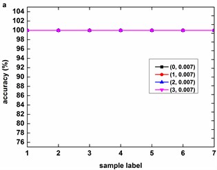
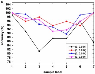
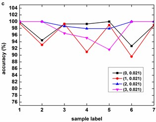
The classification accuracy of KMCSVM is observed as the fault size changes under specific loads (0 HP, 1 HP, 2 HP, 3 HP). It can be inferred from Fig. 7 that the accuracy of KMCSVM descends in sequence of fault sizes from 0.007 to 0.021 then to 0.014 inch except that the accuracy alternately occurs between 0.014 and 0.021 inch under 1 HP load as described Fig. 7(b). In the early stage of bearing fault (0.007 inch), the accuracy arrives at 100 %. The accuracy then falls with the growth of bearing fault (0.014 inch). When the fault size further enlarges (0.021 inch), the classification accuracy rises again.
Fig. 6Accuracy of the four classifiers corresponding to 12 datasets
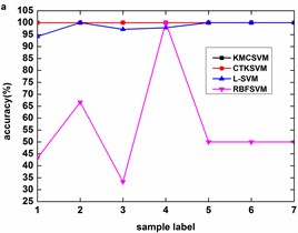
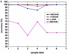
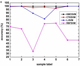

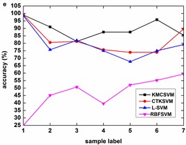
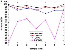
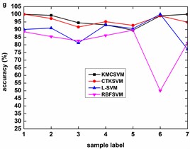
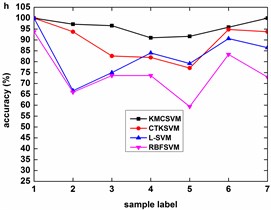
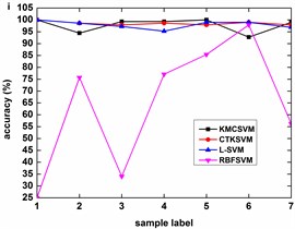
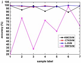
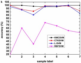
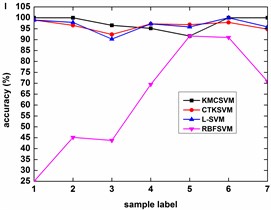
Fig. 8 describes the classification accuracy of KMCSVM with the load variation while fixing the fault size. In Fig. 8(a), the accuracy for fault with 0.007 inch always keeps 100 %. So KMCSVM is robust against the load interference and excellent fault classification performance. From Fig. 8(b) and Fig. 8(c), it demonstrates that the loading disturbances bring the accuracy fluctuations irregularly.
It also can be seen from Table 6 that the average accuracy of KMCSVM, whenever five-fold cross validation or independent test, is the highest (all more than 95.60 %). The corresponding training and test time are summarized in Table 7. For 5 folds cross validation, the computational cost of training KMCSVM is higher than that of the other three methods. The reason is that the construction of training kernel matrix needs more computational time. Once KMCSVM is trained, it has the efficient diagnosis capability with no more than 8.3 s. For independent validation, it takes less time to train (less than 9.97 s) and test (less than 3.02 s) KMCSVM which is very close to other methods. Thereby, KMCSVM displays its outstanding fault diagnosis performance.
Fig. 7Accuracy of KMCSVM with the fault size variation
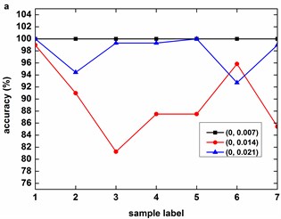
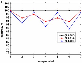
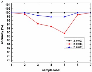
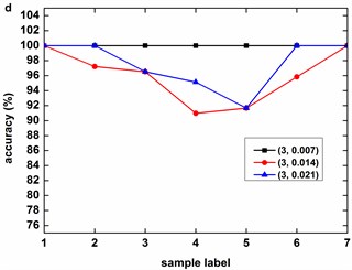
Fig. 8Accuracy of KMCSVM with the load variation
4.3.2. Identification of fault severity
Fault severity recognition seeks to evaluate REB fault size that influences the machinery health and its lifetime. In Table 8, four types of fault severity conditions are considered to assess KMCSVM classification performance using datasets in Table 9.
The groups of sample sets are provided by means of tournament to identify different fault sizes as described in Table 10.
Table 6Average accuracy of 4 classifiers using 12 datasets on fault locations
Sample set | 5 folds cross validation | Independent validation | ||||||
KMCSVM | CTKSVM | L-SVM | RBFSVM | KMCSVM | CTKSVM | L-SVM | RBFSVM | |
H vs. (O+I+B) | 99.87 | 99.57 | 97.79 | 49.01 | 99.65 | 99.39 | 93.75 | 44.44 |
O vs. (I+B) | 97.57 | 95.95 | 92.59 | 66.38 | 97.68 | 95.60 | 92.59 | 68.06 |
B vs. (O+I) | 96.99 | 93.87 | 89.12 | 48.15 | 96.41 | 93.52 | 87.50 | 62.38 |
I vs. (O+B) | 95.72 | 94.04 | 90.58 | 72.34 | 95.60 | 94.10 | 84.49 | 74.19 |
I vs. B | 96.09 | 93.84 | 92.45 | 66.84 | 95.66 | 92.36 | 92.19 | 58.16 |
O vs. I | 97.22 | 96.34 | 96.09 | 64.18 | 97.40 | 96.35 | 95.83 | 56.42 |
O vs. B | 98.61 | 96.53 | 92.53 | 63.37 | 98.26 | 96.18 | 93.39 | 69.44 |
Table 7Average training time and test time of 4 classifiers using 12 datasets on fault locations
Sample set | Time (s) | 5 folds cross validation | Independent validation | ||||||
KMCSVM | CTKSVM | L-SVM | RBFSVM | KMCSVM | CTKSVM | L-SVM | RBFSVM | ||
H vs. (O+I+B) | Train | 262.73 | 12.86 | 10.75 | 15.82 | 9.97 | 1.90 | 1.57 | 4.97 |
Test | 8.30 | 0.01 | 0.01 | 0 | 3.02 | 0 | 0 | 0 | |
O vs. (I+B) | Train | 108.29 | 11.94 | 10.76 | 12.87 | 3.96 | 1.98 | 1.60 | 3.11 |
Test | 5.90 | 0 | 0 | 0 | 1.25 | 0 | 0 | 0 | |
B vs. (O+I) | Train | 109.28 | 14.42 | 11.95 | 14.27 | 3.93 | 2.10 | 1.76 | 3.16 |
Test | 5.54 | 0 | 0 | 0 | 1.25 | 0 | 0 | 0 | |
I vs. (O+B) | Train | 107.91 | 14.31 | 11.93 | 13.80 | 4.14 | 2.12 | 1.93 | 3.35 |
Test | 5.23 | 0 | 0 | 0 | 1.28 | 0 | 0 | 0 | |
I vs. B | Train | 33.66 | 9.76 | 8.45 | 9.29 | 1.22 | 1.55 | 1.35 | 1.76 |
Test | 1.51 | 0 | 0 | 0 | 0.42 | 0 | 0 | 0 | |
O vs. I | Train | 29.03 | 8.51 | 7.40 | 8.30 | 1.42 | 1.44 | 1.28 | 1.71 |
Test | 1.39 | 0 | 0 | 0 | 0.40 | 0 | 0 | 0 | |
O vs. B | Train | 28.54 | 9.53 | 8.09 | 8.97 | 1.31 | 1.55 | 1.41 | 1.83 |
Test | 1.38 | 0 | 0 | 0 | 0.40 | 0 | 0 | 0 | |
Table 8Composition of dataset on fault severity
Fault severity | Sample size | Defect size(inch) |
H | 48 | 0 |
S1 | 48 | 0.007 |
S2 | 48 | 0.014 |
S3 | 48 | 0.021 |
H – healthy, S1 – fault with 0.007 inch, S2 – fault with 0.014 inch, S3 – fault with 0.021 inch | ||
Table 9Description of 12 datasets on fault severity
Dataset | 1 | 2 | 3 | 4 | 5 | 6 | 7 | 8 | 9 | 10 | 11 | 12 |
Location | O | O | O | O | I | I | I | I | B | B | B | B |
Load (HP) | 0 | 1 | 2 | 3 | 0 | 1 | 2 | 3 | 0 | 1 | 2 | 3 |
Speed (RPM) | 1796 | 1772 | 1750 | 1725 | 1796 | 1772 | 1750 | 1725 | 1796 | 1772 | 1750 | 1725 |
Fig. 9, Fig. 10 and Fig. 11 illustrate the accuracy of KMCSVM tested on the 12 datasets in Table 6 using five-fold cross validation and compared with CTKSVM, L-SVM and RBFSVM. Clearly, RBFSVM contributes to the lowest accuracy. In seven cases (Fig. 9(a)-(d) and Fig. 10(a)-(c)), KMCSVM reaches the highest 100 %. In four cases Fig. 10(d), Fig. 11(a) and Fig. 11(c)-(d)), the accuracy based on KMCSVM are second only to L-SVM. Fig. 11(b) indicates the accuracy of KMCSVM is slightly lower than those of CTKSVM and L-SVM. Consequently, KMCSVM is highly suitable for fault severity recognition of bearing outer race and inner race. Moreover, the accuracy curves of KMCSVM stay little fluctuation. It exhibits good stability of KMCSVM on changes of sample sets and load interference.
Fig. 9Accuracy of the four classifiers for fault severity in bearing outer race
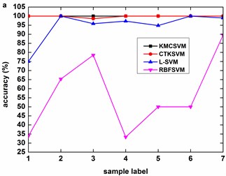
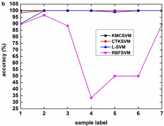
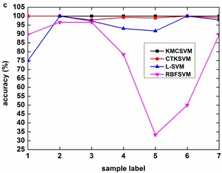
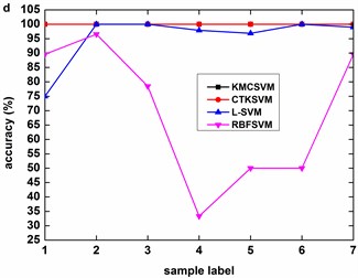
Fig. 10Accuracy of the four classifiers for fault severity in bearing inner race
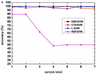
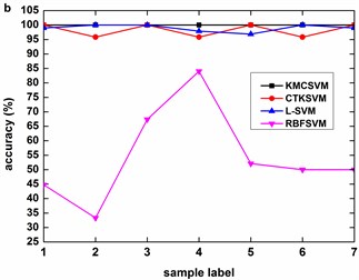
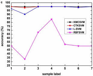
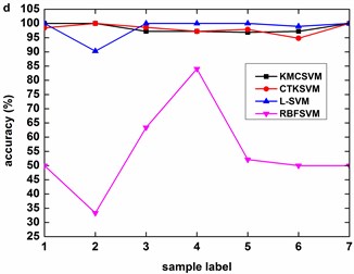
Table 11 gives the average accuracy of 4 classifiers about REB fault severity recognition. For five-fold cross validation, the classification performance of KMCSVM is slightly lower than L-SVM because KMCSVM is not so well as L-SVM in fault severity recognition of bearing ball. However, KMCSVM is the best one of 4 classifiers which gets the highest accuracy for independent test. The corresponding training and test time are shown in Table 12. The computational cost of training and test KMCSVM is similar to that used for fault locations diagnosis mentioned above.
Fig. 11Accuracy of the four classifiers for fault severity in bearing ball
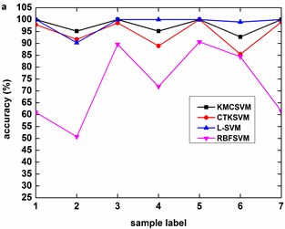
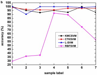
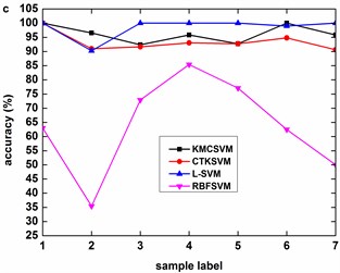
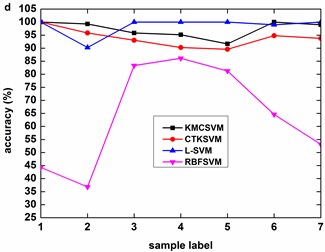
Table 10Sample set with different severities for training and test
Sample label | 5 folds cross validation | Independent test | ||
Training | Test | |||
1 | H vs. (S1+S2+S3) | 48: (48 + 48 + 48) | 24: (24 + 24 + 24) | 24: (24 + 24 + 24) |
2 | S1 vs. (S2+S3) | 48: (48 + 48) | 24: (24 + 24) | 24: (24 + 24) |
3 | S3 vs. (S1+S2) | 48: (48 + 48) | 24: (24 + 24) | 24: (24 + 24) |
4 | S2 vs. (S1+S3) | 48: (48 + 48) | 24: (24 + 24) | 24: (24 + 24) |
5 | S2 vs. S3 | 48:48 | 24: 24 | 24: 24 |
6 | S1 vs. S2 | 48:48 | 24: 24 | 24: 24 |
7 | S1 vs. S3 | 48:48 | 24: 24 | 24: 24 |
Table 11Average accuracy of 4 classifiers using 12 datasets on fault severity
Sample set | 5 folds cross validation | Independent validation | ||||||
KMCSVM | CTKSVM | L-SVM | RBFSVM | KMCSVM | CTKSVM | L-SVM | RBFSVM | |
H vs. (S1+S2+S3) | 100 | 99.48 | 92.54 | 61.24 | 99.74 | 99.13 | 80.73 | 83.42 |
S1 vs. (S2+S3) | 98.84 | 97.28 | 95.14 | 58.62 | 98.73 | 92.94 | 83.91 | 80.44 |
S3 vs. (S1+S2) | 98.15 | 97.79 | 99.42 | 74.17 | 98.03 | 96.76 | 92.13 | 85.07 |
S2 vs. (S1+S3) | 98.21 | 96.59 | 98.67 | 67.85 | 97.80 | 93.12 | 86.81 | 82.87 |
S2 vs. S3 | 97.83 | 98.10 | 98.00 | 60.68 | 97.57 | 96.89 | 92.19 | 90.11 |
S1 vs. S2 | 99.16 | 96.70 | 99.48 | 57.12 | 98.79 | 93.75 | 88.02 | 84.03 |
S1 vs. S3 | 98.96 | 98.09 | 99.48 | 65.02 | 99.13 | 98.96 | 94.27 | 80.21 |
According to the results in the above experiments, KMCSVM earns higher accuracy in diagnosis of fault locations and severities compared to the other three methods. The success of KMCSVM owes to the strategy for the construction of kernel matrix and . This strategy can effectively suppress irrelevant features and mine the similarity degree of samples. So and can express the intra-class compactness and inter-class separation more objectively than CTKSVM. RBFSVM and L-SVM employ fixed kernels that have nothing to do with the analyzed samples, thus fall behind KMCSVM and CTKSVM. Hence, KMCSVM is a competitive method for REB fault diagnosis.
Table 12Average training time and test time of 4 classifiers using 12 datasets on fault severity
Sample set | Time (s) | 5 folds cross validation | Independent validation | ||||||
KMCSVM | CTKSVM | L-SVM | RBFSVM | KMCSVM | CTKSVM | L-SVM | RBFSVM | ||
H vs. (S1+S2+S3) | Train | 164.32 | 11.75 | 10.68 | 15.84 | 15.58 | 1.87 | 1.53 | 3.76 |
Test | 5.86 | 0.01 | 0 | 0.01 | 5.08 | 0 | 0 | 0 | |
S1 vs. (S2+S3) | Train | 66.69 | 11.82 | 10.56 | 12.46 | 6.62 | 1.91 | 1.55 | 2.53 |
Test | 5.42 | 0 | 0.01 | 0 | 2.07 | 0 | 0 | 0 | |
S3 vs. (S1+S2) | Train | 63.68 | 11.51 | 9.60 | 11.60 | 6.44 | 1.74 | 1.43 | 2.38 |
Test | 5.54 | 0 | 0 | 0 | 2.15 | 0 | 0 | 0 | |
S2 vs. (S1+S3) | Train | 61.69 | 12.16 | 10.27 | 12.42 | 6.49 | 1.89 | 1.56 | 2.47 |
Test | 5.22 | 0 | 0 | 0 | 2.16 | 0 | 0 | 0 | |
S2 vs. S3 | Train | 17.85 | 8.74 | 7.38 | 8.52 | 2.14 | 1.52 | 1.26 | 1.53 |
Test | 0.98 | 0 | 0 | 0 | 0.65 | 0 | 0 | 0 | |
S1 vs. S2 | Train | 17.30 | 9.24 | 7.89 | 8.97 | 2.10 | 1.53 | 1.30 | 1.60 |
Test | 1.03 | 0 | 0 | 0 | 0.64 | 0 | 0 | 0 | |
S1 vs. S3 | Train | 17.02 | 7.78 | 6.72 | 7.73 | 2.30 | 1.35 | 1.16 | 1.45 |
Test | 0.95 | 0 | 0 | 0 | 0.67 | 0 | 0 | 0 | |
5. Conclusions
In this study, KMCSVM based on kernel matrix construction is proposed to carry out nonlinear classification for REB defects. The results of fault locations and severities identification verify that KMCSVM can achieve higher accuracy for bearing fault diagnosis than the other SVM classifiers. KMCSVM also has the ability to keep robust against the load interferences and detects defects at earlier time, which is significant for REB condition monitoring. In addition, the effectiveness of KMCSVM can help to predict deterioration degree and remaining lifetime of bearing. Summarily, KMCSVM demonstrates its great advantages and potential in rotating machinery fault diagnosis.
References
-
Lou X. S., Loparo K. A. Bearing fault diagnosis based on wavelet transform and fuzzy inference. Mechanical Systems and Signal Processing, Vol. 18, Issue 5, 2004, p. 1077-1095.
-
Safizadeh M. S., Latifi S. K. Using multi-sensor data fusion for vibration fault diagnosis of rolling element bearings by accelerometer and load cell. Information Fusion, Vol. 18, 2014, p. 1-8.
-
Fan Z. Q., Li H. Z. A hybrid approach for fault diagnosis of planetary bearings using an internal vibration sensor. Measurement, Vol. 64, 2015, p. 71-80.
-
Saucedo-Espinosa M. A., Escalante H. J., Berrones A. Detection of defective embedded bearings by sound analysis: a machine learning approach. Journal of Intelligent Manufacturing, Vol. 28, Issue 2, 2017, p. 489-500.
-
El-Thalji I., Jantunen E. A summary of fault modelling and predictive health monitoring of rolling element bearings. Mechanical Systems and Signal Processing, Vols. 60-61, 2015, p. 252-272.
-
Wu C. X., Chen T. F., Jiang R., Ning L. W., Jiang Z. ANN based multi-classification using various signal processing techniques for bearing fault diagnosis. International Journal of Control and Automation, Vol. 8, Issue 7, 2015, p. 113-124.
-
Samanta B., Al Balushi K.-R. Artificial neural network based fault diagnostics of rolling element bearings using time-domain features. Mechanical Systems and Signal Processing, Vol. 17, Issue 2, 2003, p. 317-328.
-
Cheng J. S., Yu D. J., Yang Y. A fault diagnosis approach for roller bearings based on EMD method and AR model. Mechanical Systems and Signal Processing, Vol. 20, Issue 2, 2006, p. 350-362.
-
Wang C. C., Kang Y., Shen P. C., Chang Y. P., Chung Y. L. Applications of fault diagnosis in rotating machinery by using time series analysis with neural network. Expert Systems with Applications, Vol. 37, Issue 2, 2010, p. 1696-1702.
-
Li H. K., Lian X. T., Guo C., Zhao P. S. Investigation on early fault classification for rolling element bearing based on the optimal frequency band determination. Journal of Intelligent Manufacturing, Vol. 26, Issue 1, 2015, p. 189-198.
-
Rai V. K., Mohanty A. R. Bearing fault diagnosis using FFT of intrinsic mode functions in Hilbert-Huang transform. Mechanical Systems and Signal Processing, Vol. 21, Issue 6, 2007, p. 2607-2615.
-
Tsao W. C., Li Y. F., Le D. D., Pan M. C. An insight concept to select appropriate IMFs for envelop analysis of bearing fault diagnosis. Measurement, Vol. 45, Issue 6, 2012, p. 1489-1498.
-
Dong G. M., Chen J., Zhao F. G. A frequency-shifted bispectrum for rolling element bearing diagnosis. Journal of Sound and Vibration, Vol. 339, 2015, p. 396-418.
-
Xue X. M., Zhou J. Z., Xu Y. H., Zhu W. L., Li C. S. An adaptively fast ensemble empirical mode decomposition method and its applications to rolling element bearing fault diagnosis. Mechanical Systems and Signal Processing, Vol. 62, Issue 63, 2015, p. 444-459.
-
Yan R. Q., Gao R. X., Chen X. F. Wavelets for fault diagnosis of rotary machines: a review with applications. Signal Processing, Vol. 96, 2014, p. 1-15.
-
Li C., Liang M. A generalized synchrosqueezing transform for enhancing signal time-frequency representation. Signal Processing, Vol. 92, Issue 9, 2012, p. 2264-2274.
-
Ali J. B., Fnaiech N., Saidi L., Chebel-Morello B., Fnaiech F. Application of empirical mode decomposition and artificial neural network for automatic bearing fault diagnosis based on vibration signals. Applied Acoustics, Vol. 89, 2015, p. 16-27.
-
Patel V. N., Tandon N., Pandey R. K. Defect detection in deep groove ball bearing in presence of external vibration using envelope analysis and Duffing oscillator. Measurement, Vol. 45, Issue 5, 2012, p. 960-970.
-
Pandya D. H., Upadhyay S. H., Harsha S.P. Fault diagnosis of rolling element bearing with intrinsic mode function of acoustic emission data using APF-KNN. Expert Systems with Applications, Vol. 40, Issue 10, 2013, p. 4137-4145.
-
Wang Z. J., Han Z. N., Gu F. S., Gu J. X., Ning S. H. A novel procedure for diagnosing multiple faults in rotating machinery. ISA Transactions, Vol. 55, 2015, p. 208-218.
-
Kankar P. K., Sharma S. C., Harsha S. P. Fault diagnosis of ball bearings using continuous wavelet transform. Applied Soft Computing, Vol. 11, Issue 2, 2011, p. 2300-2312.
-
Rafiee J., Tse P. W., Harifi A., Sadeghi M. H. A novel technique for selecting mother wavelet function using an intelligent fault diagnosis system. Expert Systems with Applications, Vol. 36, Issue 3, 2009, p. 4862-4875.
-
Zhang C. L., Li B., Chen B. Q., Cao H. R., Zi Y. Y., He Z. J. Weak fault signature extraction of rotating machinery using flexible analytic wavelet transform. Mechanical Systems and Signal Processing, Vol. 64, Issue 65, 2015, p. 162-187.
-
Saravanan N., Siddabattuni V. N. S. K., Ramachandran K. I. Fault diagnosis of spur bevel gear box using artificial neural network (ANN) and proximal support vector machine (PSVM). Applied Soft Computing, Vol. 10, Issue 1, 2010, p. 344-360.
-
Konar P., Chattopadhyay P. Bearing fault detection of induction motor using wavelet and support vector machines (SVMs). Applied Soft Computing, Vol. 11, Issue 6, 2011, p. 4203-4211.
-
Gan M., Wang C., Zhu C. A. Multiple-domain manifold for feature extraction in machinery fault diagnosis. Measurement, Vol. 75, 2015, p. 76-91.
-
Tang B. P., Song T., Feng Li, Deng L. Fault diagnosis for a wind turbine transmission system based on manifold learning and Shannon wavelet support vector machine. Renewable Energy, Vol. 62, 2014, p. 1-9.
-
Gharavian M. H., Ganj F. A., Ohadi A. R., Bafroui H. H. Comparison of FDA-based and PCA-based features in fault diagnosis of automobile gearboxes. Neurocomputing, Vol. 121, 2013, p. 150-159.
-
Li F., Tang B., Yang R. S. Rotating machine fault diagnosis using dimension reduction with linear local tangent space alignment. Measurement, Vol. 46, Issue 8, 2013, p. 2525-2539.
-
Zhao M. B., Jin X. H., Zhang Z., Li B. Fault diagnosis of rolling element bearings via discriminative subspace learning: visualization and classification. Expert Systems with Applications, Vol. 41, Issue 7, 2014, p. 3391-3401.
-
Kan M. S., Tan A. C. C., Mathew J. A review on prognostic techniques for non-stationary and non-linear rotating systems. Mechanical Systems and Signal Processing, Vol. 62, Issue 63, 2015, p. 1-20.
-
Purarjomandlangrudi A., Ghapanchi A. H., Esmalifalak M. A data mining approach for fault diagnosis: An application of anomaly detection algorithm. Measurement, Vol. 55, 2014, p. 343-352.
-
Tamilselvan P., Wang P. F. Atri-fold hybrid classification approach for diagnostics with unexampled faulty states. Mechanical Systems and Signal Processing, Vol. 50, Issue 51, 2015, p. 437-455.
-
Ali J. B., Chebel-Morello B., Saidi L., Malinowski S., Fnaiech F., Accurate bearing remaining useful life prediction based on Weibull distribution and artificial neural network. Mechanical Systems and Signal Processing, Vol. 56, Issue 57, 2015, p. 150-172.
-
Yunusa-Kaltungo A., Sinha J. K., Elbhbah K. An improved data fusion technique for faults diagnosis in rotating machines. Measurement, Vol. 58, 2014, p. 27-32.
-
Saidi L., Ali J. B., Fnaiech F. Application of higher order spectral features and support vector machines for bearing faults classification. ISA Transactions, Vol. 54, 2015, p. 193-206.
-
Wu C. X., Chen T. F., Jiang R., Ning L. W., Jiang Z. A novel approach to wavelet selection and tree kernel construction for diagnosis of rolling element bearing fault. Journal of Intelligent Manufacturing, 2015, https://doi.org/10.1007/s10845-015-1070-4.
Cited by
About this article

The work was supported by National High Technology Research and Development Program of China (2009AA11Z217). The authors would like to thank all the reviewers for giving valuable comments and constructive suggestions on this paper. The authors also thank Case Western Reserve University for downloading the bearing data freely.
