Abstract
With the development of theoretical models, numerical algorithms and available computational power, numerical aero-acoustics presents a huge prospect for solving the actual problems of aerodynamic noises. Under low Mach number, structures with a complicated geometric shapes were selected as the research objects to analyze their aerodynamic noises by means of flow-sound separation algorithm based on immersed boundary method. Firstly, the incompressible complicated flow field was solved on the basis of immersed boundary method, and the flow field parameters were obtained as the input values. Then, the linear compressible perturbation equation was solved to simulate generation and travel of acoustic waves. This method was used to predict the noise of flow past two circular cylinders in tandem arrangements and the aerodynamic noise of the rudimentary landing gear. The numerical simulation was then compared with the corresponding experiments, and results were consistent. That showed the algorithm proposed was feasible.
1. Introduction
The computational aero-acoustics has been successfully applied to many aerodynamic noise problems. For instance, the direct noise algorithm can be used to solve the jet noises [1, 2]. Airframe noise which should be critically considered when it is designed [3]. For this problem, many researchers researched airframe noises by taking the standard shapes and airfoil profiles as the research objects [3-9]. However, due to that the Mach number ( 0.3) was low and the geometric profile was complicated, some actual airframe noise problems including the landing gear noise haven’t been solved completely [10, 11]. The computational aero-acoustics (CAA) had the following several methods for dealing with the complicated geometric profile, which were block-structured grid method [12], overlapping structured grid method [13, 14] and finite volume method [15-18] as well as immersed boundary method (IBM) [19-23]. The front two methods had some limitations in solving the complicated geometric profile, while DGM needed high computational costs. IBM (Reference [24]) was a universal method for dealing with the complicated geometric profile. A problem of the complicated geometric profile can be solved based on Cartesian grid by using IBM. As it was based on Cartesian grid, the perfect and high-efficient finite difference technique can be used.
Recently, researchers proposed a method for solving aero-acoustics problem of the complicated geometric profile and low Mach number by using an algorithm which based on hydrodynamic force and sound separation technology [25-27]. In this method, the flow field information can be acquired by solving the incompressible N-S equation (INS). And the sound field can be predicted by the linear compressible perturbation equation (LPCE). INS/LPCE hybrid technology was a coupling method to directly simulate flow noise. The incompressible flow filed solver which was based on IBM was adopted to solve the complicated LPCE equations in the paper. The virtual element technology was adopted in this IBM [28, 29]. Luo [30] initially put forward to expand this method to a higher order by using the approaching multinomial. With this method, Dirichlet boundary conditions and Neumann boundary conditions with a high accuracy can be realized on the solid wall surface. Therefore, the dispersion and dissipation caused by boundary condition can be minimized, so as to further ensure the precise expression of sound wave on the wall. In this paper, this method was applied to calculate the aerodynamic noises of the objects with the complicated geometric profile to verify its reliability.
2. Algorithms
2.1. Control equations
In this paper, the hybrid method which was based on hydrodynamic force and sound separation [25, 26] was adopted to directly calculate aerodynamic noise under low Mach number. All flow variables were decomposed into the incompressible parts and compressible perturbation parts in this method:
Control equations of the incompressible part was N-S equation (INS), which represented flow field information and sound pulsation. And the other compressible effects were expressed by perturbation variable (). N-S equation was written as follow:
Sound perturbation variables can be acquired by solving the linearized compressible perturbation equation (LPCE) after obtaining the incompressible flow solution [27]. The vector of LPCE equation can be written as follow:
INS/LPCE hybrid method has been successfully verified by the basic acoustic problems such as dipole and quadrupole [27]. Meanwhile, it was also applicable to turbulent flow noise problem [7, 9]. The left side of LPCE equation indicated the propagation and emission of sound waves, while its right side only included sound source item.
2.2. Numerical method
The incompressible N-S Eq. (3) was solved by several steps. The spatial derivatives were handled by two order central difference [28]. Pressure Poisson equation was solved by means of multiple grid method based on Line-Gauss-Seidel (LGS) matrix. LPCE spatial discretization was subject to six-order compact central difference [31], and time integral was subject to four-order Runge-Kutta. Three-order and four-order boundary were adopted near the immersed solid boundary [31]. The implicit spatial filtering [32] was adopted to restrain the high frequent errors, because there was no dissipation error in compact central difference. Ten-order filtering was adopted in the internal areas in the paper, and the filtering near the boundaries reduced to two-order from eight-order successively. The compact central difference and filtering format of implicit spatial can be solved by means of a tridiagonal matrix.
2.3. Immersed boundary method
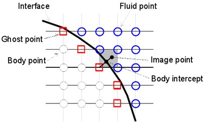
The flow problems of the complicated immersed boundaries were solved by the incompressible N-S equation [28]. In this method, the surface of the immersed object was indicated by the unstructured surface grid of triangular elements. Before integral for control equations, all the elements inside the object were marked as “body points”, and the other points outside the object were marked as “fluid points”. Any element which was near fluid elements was marked as “image point”, as shown in Fig. 1(a). Wall boundary conditions were realized by assigning proper values for the image points, as shown in Fig. 1(b).
Fig. 1a) Diagram of image points and b) diagram of boundary conditions
a)
b)
The higher order immersed boundary method [23] adopted in sound solution was high order polynomial interpolation which was based on weighted Least Squares Error. Image point values determined whether it met the boundary conditions at Body Intercept (BI) points. In particular, a general variable which was near BI points was estimated by using -order polynomial:
where, , , , was an unknown coefficient and was expressed as follows:
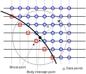
Sizes of coefficients for three-order polynomial ( 3) was 10 and 20 under two-dimensional and three-dimensional conditions, respectively. Coefficients of polynomials with different orders were described in reference [23]. To determine these coefficients, the data of the flow field points near BI points needed to be acquired. According to method of Luo [30], the flow field values in the circle or ball (under three-dimensional conditions) with the object point as the center and the radius of can be selected as the data. For data points, coefficient was determined by the minimum weighted error estimation:
where, was the th data point, was weight function. According to experience of the previous researchers [30], cosine weight function was used in this paper. To make the least square problem appropriate, radius should be selected in an appropriate way which can ensure that there were more sizes of data points than that of coefficients. To find the values of image points and BI points, the first data point was a image point, the other (1) data points shall be found in the fluid region (as shown in Fig. 1(b)). The precise solution of least square problem (Eq. (9)) was as follow:
where the superscript “+” indicated the generalized inverse of matrix, vector and included coefficient and data , respectively. and indicated weight matrix and Vandermonde matrix, respectively. indicated the first image point. Coefficient can be written as the linear combination of after solving Eq. (10). According to Eq. (8), coefficient indicated the value and derivative value of :
Therefore, for Dirichlet and Neumann boundary conditions given on wall surface, Image point values can be acquired by Eq. (10) and Eq. (11). The details of the equation for immersed boundary conditions can refer to reference [23].
2.4. Disposing the freshly cleared point
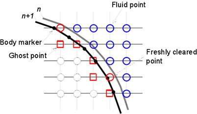
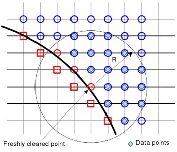
Disposing the moving object on the fixed grid would generate “freshly cleared points”, as shown in Fig. 2(a). As the time-dependent variable values of the freshly cleared points did not need to participate in integral of control equations, they can be obtained through interpolation among the near elements [33]. In solving the incompressible flow, the variable values of the new time layer were acquired by iteration of the momentum equation [28]. In solving acoustic solution, the values of the freshly cleared points were acquired through the high order multinomial Eq. (7). The entire assignment process was similar to the disposal of image points in Section 2.3. However, for freshly cleared points, the center of the data points was the freshly cleared point , where , , , as shown in Fig. 2(b). To avoid iteration, only the non-updated elements and fluid elements are selected as the data points to minimize Least Squares Error. Solving Eq. (10) will acquire the coefficient of the approaching multinomial, and then the value of the updated element can be directly given by the first coefficient, for instance:
3. Results and discussions
The mentioned methods have successfully applied to calculating noise of flow around a circular cylinder under laminar flow conditions. The effectiveness of the methods has been verified by comparing its results with that of the direct noise based on the compressible N-S equation [23]. Noise of two tandem circular cylinders was the basic model for researching airframe noise. The method was expanded to calculating the flow noise problems of two tandem circular cylinders under turbulent flow status in the paper. Meanwhile, to verify the solving ability of this method for the complicated profile, the flow noise of the rudimentary landing gear model was calculated by it.
Fig. 2a) Diagram of moving boundary and b) diagram of disposal for the freshly cleared point
a)
b)
3.1. Turbulent flow noise of two tandem circular cylinders
As shown in Fig. 3, the mentioned method was applied to calculating the flow-induced noise of two tandem circular cylinders. This problem was a standard calculation example for researching airframe noise [34]. The inflow velocity 44 m/s, and the corresponding Reynolds number 1.66×10⁵. Mach number 0.128 was suitable for the hybrid algorithm. During computing noise by means of this method, the computational domain size was 3040, –4040. And span-wise length . The periodic boundary condition was applied in the span-wise direction. Sizes of the non-homogeneous Cartesian grids were 768×384×32. Fig. 4 showed the computational result in - plane. The periodic boundary conditions were not marked in the figure, and it can be easily understood. We cared more about the cylinder wake vortex shedding and its mutual influences, and the periodic boundary conditions were applied to up, down, left and right planes in the computational domain. This was a very conventional method used in three-dimensional computation:
where and were the vortex and strain rate tensor, respectively. Under the current Reynolds number, the distance between the two circular cylinders was 3.7. The wake flow of the upstream circular cylinder was in rolling up status before arriving at the downstream circular cylinder. The shedding vortex of the upstream circular cylinder and that of the downstream circular cylinder interacted with each other. The characteristics of the entire flow field were similar to that of the higher Reynolds number [35]. The change curve of aerodynamic coefficient with time was shown in Fig. 5. The coefficient average value and mean square root (rms) was shown in Table 1. It was shown that the aerodynamic force fluctuation of the downstream circular cylinder was more serious, because of the interference of the shedding vortex of the upstream circular cylinder. The main frequency of vortex shedding was 0.196. The aerodynamic force was higher than that of the experimental result under the higher Reynolds number (1.66×10⁵) [34-36]. Although the shedding frequency (0.196) was lower than the experimental result of NASA [36-38] (0.234), it was very close to the direct numerical simulation result (0.18, 1000) of Papaioannou [37] and the experimental result ( 0.19, 4000) of Igarashi.
Fig. 3Geometrical model of two tandem circular cylinders
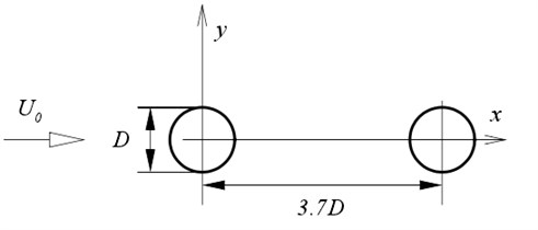
Fig. 4Vortex structure of two tandem circular cylinder
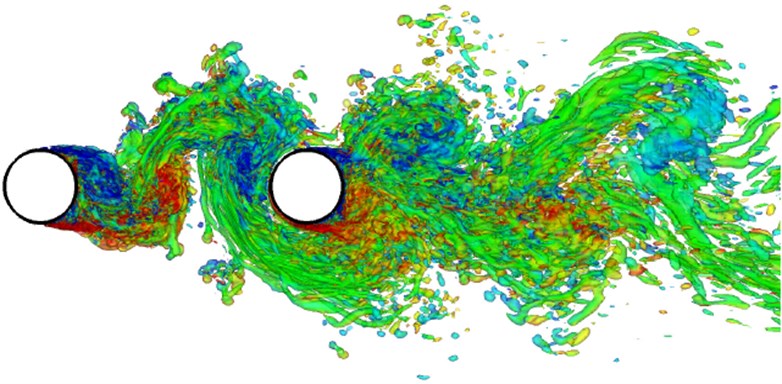
Fig. 5Change curve of aerodynamic coefficient with time
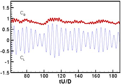
a) Upstream circular cylinder
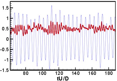
b) Downstream circular cylinder
Table 1Aerodynamic coefficient
Parameter | Upstream circular cylinder | Downstream circular cylinder |
0.849 | 0.4948 | |
0.066 | 0.1206 | |
0.364 | 0.8158 |
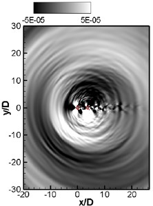
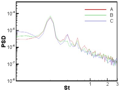
Computation of sound field was based on the incompressible flow, with LPCE as control equations. The span-wise was assumed to be periodic during computing the flow field. As scale of the sound wave length was larger than flow scale under current Mach number (0.128), span-wise length was not enough to computer three-dimensional sound field. Based on the research of Seo [7], three-dimensional sound field was directly related to the central plane in span-wise direction, as a result, the two-dimensional sound field at zero span-wise direction () was computed. The computational result was modified to three-dimension by Oberai formula [39]. The contour line of time-average expansion rate for sound field was shown in Fig. 6(a). It can be observed that the wave-length of the main frequency sound wave was approximate 40.5, and the high frequency components caused by turbulent fluctuation can also be observed. The sound pressures were observed at three points, which were (–8.33, 27.815), (9.11, 32.49) and (26.55, 27.815), respectively. The positions of the observation points were the same as that of the sensors arranged in NASA experiment. The power spectral density of the sound pressure pulsation at each observation point was shown in Fig. 6(b). The spectrogram was promoted to the central plane data of three-dimensional result through modification [7]. Sound pressure frequency spectrum was constituted of broadband noise and pure tones with large amplitudes at main frequency. It was consistent with the experimental data [36]. The computational domain in - plane of sound field was kept consistent with that of the flow field, the grid size was 500×400. The grid resolution near sound field was as twice as that of the flow field. It was more accurate at far field to accurately distinguish the high frequency sound waves.
Fig. 6a) Contour line of the instantaneous expansion rate of sound field and b) the power spectral density (PSD) of sound pressure at three observation points
a)
b)
Fig. 7The power spectral density of three observation points at actual span length (16D) as modified, the solid line was the computational result, and the dot dash line with symbols was NASA experimental data [34, 36]
![The power spectral density of three observation points at actual span length (16D) as modified, the solid line was the computational result, and the dot dash line with symbols was NASA experimental data [34, 36]](https://static-01.extrica.com/articles/15813/15813-img11.jpg)
This paper attempted to compare the sound results with the experimental one. Because sound prediction was carried out under small span-wise length (), so it must be modified to the actual span-wise length () to be compared with the experimental value. This required the information related to span-wise length. In this paper, the span-wise length data provided by the experiments [34] was adopted. It was found that the length related to span-wise was longer than the span-wise length only under main shedding frequency. Based on the modification formula of Seo, the modification value of main shedding frequency was 9.4 [dB], while the other frequencies were 7.2 [dB]. The modified power spectral density and experimental result were shown in Fig. 7. Because Reynolds number of the computation was different from the experimental one, the frequency spectrum was not identical well, in particularly the wave peak and total amplitude. However, it can be found that the change trend was consistent each other. For instance, there were second-order harmonic and third-order harmonic at point A simultaneously. But third-order harmonic was obvious at point B, while second-order harmonic was obvious at point C.
3.2. Flow noise of the rudimentary landing gear
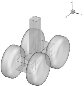
The rudimentary landing gear (RLG) model used in the present study had a modular design as shown in Fig. 8(a). The model had three main components, the vertical post, the truck, and the wheels. The model had one instrumented indexed wheel, one instrumented non-indexed wheel, and two dummy wheels. The fabrication of the landing-gear model was carried out using composites. The post was fabricated using carbon-fiber-reinforced plastics, while the truck and the wheels were fabricated using glass-fiber-reinforced plastics. Using composites for fabrication ensured that the model weight was minimal without compromising the strength of the model. The total grid number of RLG model was 187742 triangular elements.
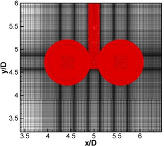
Fig. 8a) Geometric model of the rudimentary landing gear and b) Computational domain grid in x-y plane
a)
b)
Fig. 9 provided the topology and dimensions of the rudimentary landing gear model normalized with the wheel diameter . Wheel width was 0.37 and shoulder radius was 0.115. Four-wheel truck wheelbase was 1.16 and track was 0.88. Transverse axles square with side was 0.3. Longitudinal beam was 0.3 high and 0.25 wide. The vertical post was 0.25 square.
To verify the applicability of this method for complicated profiles, the flow noise of the rudimentary landing gear was calculated in this section. The computational domain was a rectangle which sizes was , , ( was the diameter of the wheel). The total number of non-uniform Cartesian grid was 512×256×256. The computational domain grid in - plane was shown in Fig. 8(b). 2000 and 0.3. Fig. 10(a) was the instantaneous vortex structure of the rudimentary landing gear. It was found that there was a complicated three-dimensional vortex structure in the wake flow area. Contour map of total pressure pulsations in different planes was shown in Fig. 10(b).
Based on flow field characteristics in Fig. 10, the sound field around the rudimentary landing gear was computed. Sound pressure levels at three observation points in Fig. 11 were extracted, as shown in Fig. 12.
Fig. 9Model topology and dimensions
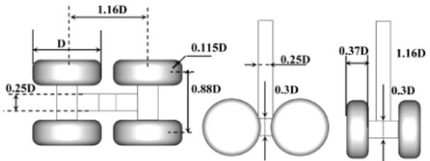
Fig. 10Instantaneous flow field and sound field
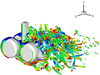
a) Vortex structure of the flow field
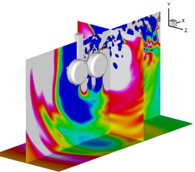
b) Contour map of total pressure pulsation
Fig. 11Positions of three observation points
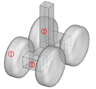
Fig. 12Sound pressure levels of three observation points
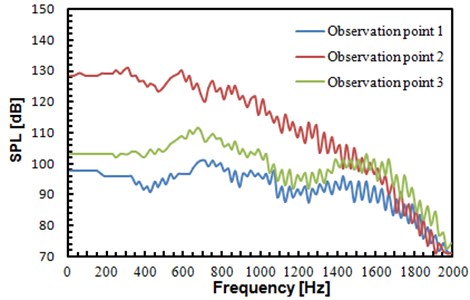
According to Fig. 12, sound pressure levels of observation point 2 was obviously higher than that of other two points. Its reasons were mainly as shown in the following. According to Fig. 10(a), the flow field of observation point 2 was relatively chaotic, while no strong flow field was formed at observation points 1 and 3. In addition, sound pressure levels of three observation points gradually decreased with the frequency increase.
Fig. 13Wind tunnel experiment of the rudimentary landing gear
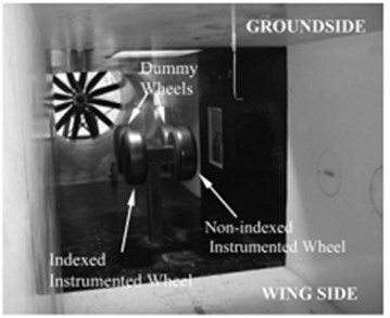
Fig. 14Testing process of flow noise for the rudimentary landing gear
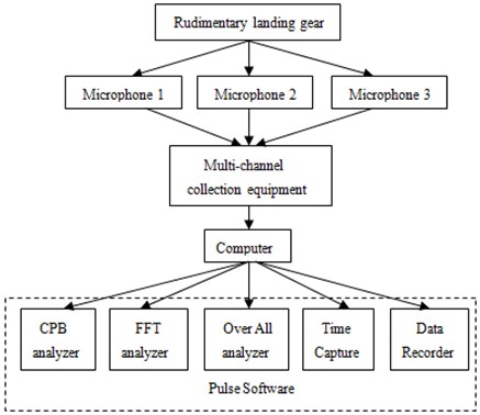
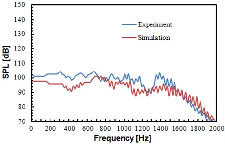
In order to verify accuracy of numerical simulation for flow noise of the rudimentary landing gear, a wind tunnel experiment was conducted, as shown in Fig. 13. The rudimentary landing gear was fixed in the wind tunnel, and an inflow with certain intensity was provided towards the rudimentary landing gear. Microphones were arranged at three points in Fig. 11. Pulse test system was used to record data. Each group of data was recorded for three times, and sampling frequency was 65536 Hz. The detailed test process was shown in Fig. 14. Sound pressure levels of the experimental were compared with the numerical simulation results, as shown in Fig. 15.
It can be found from Fig. 15 that sound pressure levels of the experimental values and that of the numerical simulation did not differ much, and the change trends were basically consistent. It was further shown in this result that the algorithm mentioned in the paper was feasible for computing the flow noise of the rudimentary landing gear.
4. Conclusions
The aerodynamic noises of structures with the complicated geometric profiles and low Mach number were computed in the paper. The flow filed and sound propagation under arbitrary motion were computed through the hybrid algorithm which included the incompressible flow field equation based on immersed boundary method and the linear compressible perturbation equation of sound field. With a good universality and applicability, this method can be used for predicting the noise of low subsonic airframe, fan noise of turbine machinery and electronic equipment. With INS/LPCE hybrid method, the basic noise problems such as dipole and quadripole can be effectively simulated, and this method was also applicable to the turbulence noise problem. In comparison with the current computational methods, this method had the following prominent characteristics. It used the right angle grid to compute flow field and sound field, and the boundary condition was simulated by means of interpolation method, which was called immersed boundary method. This method can solve the problem of the grid generation for the complicated surface, and it will cost less time for pre-processing. The further problem was about the computational accuracy of this method. Reliability of this method was verified through comparison between the computational values and the experimental one for tandem circular cylinder. According to computation and analysis of the flow noise problem for the rudimentary landing gear, feasibility of this method was also verified when it processed the complicated flow problem. In conclusion, this method was very useful to compute flow noise based on the feasibility of the actual engineering problem.
Fig. 15Comparison of sound pressure levels between experiment and simulation
a) Sound pressure levels of observation point 1
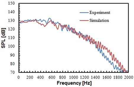
b) Sound pressure levels of observation point 2
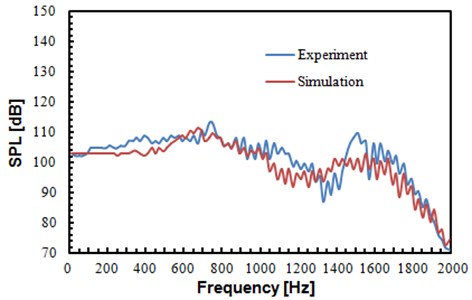
c) Sound pressure levels of observation point 3
References
-
Colonius T., Lele S. K. Computational aeroacoustics: progress on nonlinear problems of sound generation. Progress in Aerospace Sciences, Vol. 40, Issue 6, 2004, p. 345-416.
-
Bailly C., Bogey C., Marsden O. Progress in direct noise computation. International Journal of Aeroacoustics, Vol. 9, 2010, p. 123-143.
-
Lilley G. M. The prediction of airframe noise and comparison with experiment. Journal of Sound and Vibration, Vol. 239, Issue 4, 2001, p. 849-859.
-
Wang M., Moin P. Computation of trailing-edge noise using large-eddy simulation. AIAA Journal, Vol. 38, Issue 12, 2000, p. 2201-2209.
-
Ewert R., Schroder W. On the simulation of trailing edge noise with hybrid LES/APE method. Journal of Sound and Vibration, Vol. 270, Issue 3, 2004, p. 509-524.
-
Terracol M., Manoha E., Herrero C., Labourasse E., Redonnet S., Sagaut P. Hybrid methods for airframe noise numerical prediction. Theoretical and Computational Fluid Dynamics, Vol. 19, Issue 3, 2005, p.197-227.
-
Seo J. H., Moon Y. J. Aerodynamic noise prediction for long-span bodies. Journal of Sound and Vibration, Vol. 306, 2007, p. 564-579.
-
Greshner B., Thiele F., Jacob M. C., Casalino D. Prediction of sound generated by a rod-airfoil configurations using EASM DES and generalized Lighthill/FW-H analogy. Computers and Fluids, Vol. 37, Issue 4, 2008, p. 402-413.
-
Moon Y. J., Seo J. H., Bae Y. M., Roger M., Becker S. A hybrid prediction for low-subsonic turbulent flow noise. Computers and Fluids, Vol. 39, 2010, p. 1125-1135.
-
Lockard D. P., Khorrami M. R., Li F. Aeroacoustic analysis of a simplified landing gear. 9th AIAA/CEAS Aeroacoustics Conference and Exhibit, 2003, p. 2003-3111.
-
Souliez F. J., Long L. N., Morris P. J., Sharma A. Landing gear aerodynamic noise prediction using unstructured grid. International Journal of Aeroacoustics, Vol. 1, Issue 2, 2002, p. 115-135.
-
Manoha E., Guenanff R., Redonnet S., Terracol M. Acoustic scattering from complex geometries. 10th AIAA/CEAS Aeroacoustics Conference, 2004, p. 2004-2938.
-
Sherer S. E., Scott J. N. High-order compact finite difference methods on general overset grids. Journal of Computational Physics, Vol. 210, 2005, p. 459-496.
-
Sherer S. E., Visbal M. R. High-order overset-grid simulations of acoustic scattering from multiple cylinders. Proceedings of the Fourth Computational Aeroacoustics (CAA) Workshop on Benchmark Problems, NASA/CP-2004-212954, p. 255-266.
-
Hu F. Q., Hussaini M. Y., Rasetarinera P. An analysis of the discontinuous galerkin for wave propagation problems. Journal of Computational Physics, Vol. 151, 1999, p. 921-946.
-
Chevaugeon N., Hillewaert K., Gallez X., Ploumhans P., Remacle J.-F. Optimal numerical parameterization of discontinuous Galerkin method applied to wave propagation problems. Journal of Computational Physics, Vol. 223, 2007, p. 188-207.
-
Dumbser M. Munz C.-D. ADER discontinuous Galerkin schemes for aeroacoustics. C. R. Mecanique, Vol. 333, 2005, p. 683-687.
-
Toulorge T., Reymen Y., Desmet W. A 2D Discontinuous Galerkin method for aeroacoustics with curved boundary treatment. Proceedings of International Conference on Noise and Vibration Engineering, 2008, p. 565-578.
-
Cand M. 3-dimensional noise propagation using a Cartesian grid. 10th AIAA/CEAS Aeroacoustics Conference, 2004, p. 2004-2816.
-
Liu Q., Vasilyev O. V. A brinkman penalization method for compressible flows in complex geometries. Journal of Computational Physics, Vol. 227, 2007, p. 946-966.
-
Arina R., Mohammadi M. An immersed boundary method for aeroacoustics problems. 14th AIAA/CEAS Aeroacoustics Conference (29th AIAA Aeroacoustics Conference), 2008, p. 2008-3003.
-
Liu M., Wu K. Aerodynamic noise propagation simulation using immersed boundary method and finite volume optimized prefactored compact scheme. Journal of Thermal Science, Vol. 17, Issue 4, 2008, p. 361-367.
-
Seo J. H., Mittal R. A high-order immersed boundary method for acoustic wave scattering and low-mach number flow-induced sound in complex geometries. Journal of Computational Physics, Vol. 230, Issue 4, 2011, p. 1000-1019.
-
Mittal R., Iaccarino G. Immersed boundary methods. Annual Review of Fluid Mechanics, Vol. 37, 2005, p. 239-261.
-
Hardin J. C., Pope D. S. An acoustic/viscous splitting technique for computational aeroacoustics. Theoretical and Computational Fluid Dynamics, Vol. 6, 1994, p. 323-340.
-
Seo J. H., Moon Y. J. The Perturbed compressible equations for aeroacoustic noise prediction at low mach numbers. AIAA Journal, Vol. 43, Issue 8, 2005, p. 1716-1724.
-
Seo J. H. Moon Y. J. Linearized perturbed compressible equations for low Mach number aeroacoustics. Journal of Computational Physics, Vol. 218, 2006, p. 702-719.
-
Mittal R., Dong H., Bozkurttas M., Najjar F. M., Vargas A., von Loebbecke A. A versatile sharp interface immersed boundary method for incompressible flows with complex boundaries. Journal of Computational Physics, Vol. 227, 2008, p. 4825-2852.
-
Ghias R., Mittal R., Dong H. A Sharp interface immersed boundary method for compressible viscous flows. Journal of Computational Physics, Vol. 225, 2007, p. 528-553.
-
Luo H., Mittal R., Zheng X., Bielamowicz S. A., Walsh R. J., Hahn J. K. An immersed-boundary method for flow-structure interaction in biological systems with application to phonation. Journal of Computational Physics, Vol. 227, 2008, p. 9303-9332.
-
Lele S. K. Compact finite difference schemes with spectral-like resolution. Journal of Computational Physics, Vol. 103, 1992, p. 16-42.
-
Gaitonde D., Shang J. S., Young J. L. Practical aspects of higher-order accurate finite volume schemes for wave propagation phenomena. International Journal for Numerical Methods in Engineering, Vol. 45, 1999, p. 1849-1869.
-
Udaykumar H. S., Mittal R., Rampunggoon P., Khanna A. A sharp interface Cartesian grid method for simulating flows with complex moving boundaries. Journal of Computational Physics, Vol. 174, 2001, p. 345-380.
-
Lockard D. P. Tandem cylinder benchmark problem. Workshop on Benchmark Problems on Airframe Noise (BANC)-I, Problem 2: http://groups.google.com/group/afnworkshop_problem2.
-
Lockard D., Khorrami M., Choudhari M. Tandem cylinder noise predictions. 13th AIAA/CEAS Aeroacoustic Conference, 2007, p. 2007-3450.
-
Khorrami M. R., Choudhari M. M., Lockard D. P., Jenkins L. N., McGinley C. B. Unsteady flow field around tandem cylinders as prototype component interaction in airframe noise. AIAA Journal, Vol. 45, Issue 8, 2007, p. 1930-1941.
-
Papaioannou G. V., Yue D. K. P., Triantafyllou M. S., Karniadakis G. E. Three-dimensionality effects in flow around two tandem cylinders. Journal of Fluid Mechanics, Vol. 558, 2006, p. 387-413.
-
Igarashi T. Characteristics of the flow around two circular cylinders arranged in tandem, 1st report. Bulletin of JSME, Vol. B27, Issue 233, 1981, p. 2380-2387.
-
Oberai A. A., Roknaldin F., Hughes T. J. R. Trailing-Edge Noise Due to Turbulent Flows. Technical Report, No. 02-002, Boston University, 2002.
About this article

