The source localization technique based on improved functional beamforming using a virtual array

1. Introduction

Over the last decades, nearfield acoustic holography (NAH) [1, 2] and beamforming become widely studied techniques of estimating the location of the source with the microphones arrays. However, beamforming has become a popular technique to identify sound source. Conventional beamforming is a basic method that identifies the source by delaying and summing signals [3, 4]. Traditionally, the use of conventional beamforming method requires a lot of microphones and implies investing huge amounts of money in an acquisition system. Furthermore, the conventional beamforming has poor spatial resolution and the resolution would depend on the number of microphones, especially at low frequency [5].

To improve the capabilities and increase the resolution of the conventional beamforming, an improved functional beamforming method based on “virtual array” [6, 7] and functional beamforming [8, 9] is introduced. The “virtual array” can be used to avoid some constrains of beamforming methods if the sound field is assumed time stationary. The sound field could be measured by using only a few microphones, one located in a fixed position and another scanning across the “virtual array” plane. Moreover, the relative complex pressures of the sound field can be acquired by calculating the differences between two microphones. And a relative spectral matrix of the relative complex pressures measured can be calculated. Then based on the relative spectral matrix, the powerful method called improved functional beamforming with order $v$ is developed. The improved method, which relies on using a “virtual array”, can be widely used due to its low time cost, but it also can improve the accuracy of beamforming method due to the use of a matrix function of the relative spectral matrix. It also must be pointed out that the resolution of the improved method can be modified by increased the number of order $v$.

In the following sections, not only the beamforming theory is introduced but also the results of simulations and tests are presented.

2. Theory

At a first, we will give a good understanding of how the sound field information can be acquired at multiple points by using a “virtual array” and how the relative spectral matrix can be generated by measuring the relative pressure. Furthermore, a restructure solution of the Functional Beamforming (FB) based on the relative spectral matrix is introduced.

For the source localization, the most commonly used source model for producing the sound field is the monopole source. The monopole source simplest to analyze is a sphere whose amplitude varies with time. Now, assumed that the sound field can be time stationary and relative phase can be measured. Then the maximum amplitude $p_0$ will be independent of distance and time:

where the term $p$ is the complex pressure and $r$ is the distance between the microphone and the source. Due to the fact that the number of microphones used in actual measurement is limited during the measurement, the conventional beamforming method may have a poor dynamic range and low resolution especially at low frequency. To improve the capabilities and increase the resolution of the beamforming method for few microphones, an improved functional beamforming method is introduced based on a “virtual array”.

Actually, only two microphones are used by the “virtual array”. The sound field signals are sampled by the scanning one, and another fixed microphone is required to compare its phase with the scanning microphone. Then, the measured data which are sampled by the measuring and the reference microphones is analyzed by Fourier transform. Consequently, the amplitude and relative phase changes between two microphones can be obtained by computing their cross-power spectral density:

where ${\mathbf{P}}_{rel}$ is the Fourier Transform of the signal recorded by the fixed microphone and $\mathbf{P}$ represents the signal recorded by the scanning microphone in different space. The cross-power spectral density ${\mathbf{P}}^{rel}$ can be calculated so as to demonstrate that the relative pressure can be measured and be time independent. The elements of the vector ${\mathbf{P}}^{rel}$ are as followed:

According to Eq. (3) which stands for the measuring cross-correlating pressures at $M$ positions, the relative spectral matrix of the relative complex pressures measured can be defined such as:

where the operator $H$ denotes the complex conjugate transpose and $\mathbf{C}$ is the relative spectral matrix. According to Eq. (4), the relative spectral matrix $\mathbf{C}$ produced by monopole source in the free field is non-negative defined and Hermitian. The spectral decomposition of it can be written:

where $\mathbf{U}$ is a matrix whose columns, are the eigenvectors of the relative spectral matrix $\mathbf{C}$ and $\mathbf{\Sigma }$ is a diagonal matrix whose diagonal elements are the eigenvalue. Then a matrix function of the relative spectral matrix $\mathbf{C}$ is defined by:

If let $f=t^{1/v}$. Then the $v$ power of the relative spectral matrix $\mathbf{C}$ becomes:

The term $\sigma$ is the eigenvalue. An interesting thing is that the spectral matrix $\mathbf{C}$ is also related to the beamforming map defined by Conventional Beamforming (CBF) and Functional beamforming. The CBF expression is:

where, $\mathbf{w}$ is called steering vector with $M$ components. To improve the performance of this expression, assume initially that only one monopole source is existed. Let $k$ be source number. Then the relative spectral matrix $\mathbf{C}$ can be defined as:

where ${\mathbf{g}}_k$ is the array steering vector for the $k$th source, the steering vector $\mathbf{w}$ satisfies to the normalization constrain ${{\mathbf{w}}^H\mathbf{g}}_k=\text{1}$, and it can be replacing by:

where ${‖\bullet ‖}_2$ denotes $L_2$ type norm, considering that the expression of Eq. (8) is sufficiently similar to the functional beamforming, we suggest a improved functional beamforming related to the relative spectral matrix and CBF by putting Eq. (7) and Eq. (10) into Eq. (8). Finally, the output of improved functional beamforming with order v in the source area of interest is as followed:

This is the improved functional beamforming of order $v$. Typical values of v are in the range of 1-20. Applying the beamforming output with order $v$, the relative level between the beamforming sidelobes and mainlobes would be effectively increased by taking the action of the exponent on the beamforming sidelobes $t$. For monopole source, if, for example, $v=$ 1 and the beamforming output has a peak sidelobes level of –5 dB, then the improved functional beamforming with order $v=$ 2 sidelobes level will be –10 dB. The improved functional beamforming essentially eliminates sidelobes. In addition, with the use of “virtual array” technique, it improves the capabilities and increases the resolution of the beamforming method for few microphones.

3. Simulations

To demonstrate the capabilities of the improved functional beamforming with a “virtual array”, several examples are given to illustrate its prosperity by using numerical tests. In simulated experiments, model sources are located on a source plane at 0.5 m from the array plane and the reconstructed target sources domain. To facilitate the calculation and analysis, target sources domain is divided into 1 m×1 m scanning area with a grid interval of 0.1 m. And Fig. 1 presents a 6×6 “virtual array” using one reference microphone.

For the “virtual array”, only 36 virtual microphones with an interval of 0.1 m are used to measure sound pressure and relative phase can be preserved by using a fixed reference microphone. At each measured step the source signals are sampled by the measuring microphone and the reference one synchronously. Then a relative spectral matrix $\mathbf{C}$ (Eq. (4)) can be obtained by using measurement signals. Thus, the output of improved functional beamforming with order $v$ can be calculated by Eq. (11) and the monopole sources maps are presented in Figs. 2 and 3.

Fig. 1A “virtual array” using one reference microphone

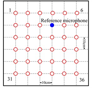
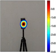
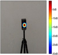
Fig. 2The numerical results of single monopole at 2.5 kHz

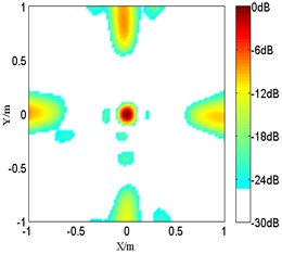
a) Improved FB with $v=$ 1

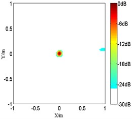
b) Improved FB with $v=$ 3

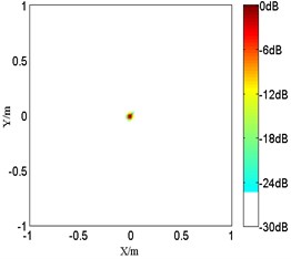
c) Improved FB with $v=$ 10

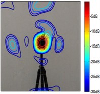
Fig. 3The numerical results of coherent sources at 1.5 kHz

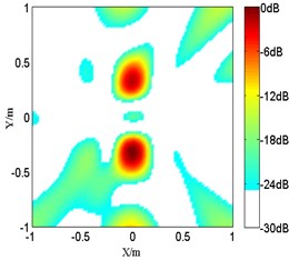
a) Improved FB with $v=$ 1

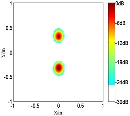
b) Improved FB with $v=$ 1

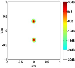
c) Improved FB with $v=$ 1

In the first problem, the monopole maps are compared among various order $v$ at 2.5 kHz in Fig. 2. And it should be mentioned that the peak values are located at the sources position. However, with a limited microphones spacing, the source map of the proposed improved functional beamforming with $v=$ 1 shows a large sidelobes around the monopole source. So the resolution of it will be too poor at high frequencies and it imposes a rather strict upper frequency limit. While the detected source spot of the proposed improved functional beamforming with a lager order $v$ becomes sharper and beamforming sidelobes are suppressed, demonstrating that the proposed improved functional beamforming with a lager order $v$ can recover the source quite well. Next, Fig. 3 compares the source maps detecting coherent sources radiating at 1.5 kHz. Similarly, the proposed improved functional beamforming, especially with a large order $v$, can recover coherent sources quite well and the size of main lobe is much narrower.

Generally, the improved functional beamforming can identify the distributed source and intensity all reasonably well both at high and low frequencies. And as the number of v increases, the improved method has a higher resolution. In other words, the proposed method can be generally better able to work in sound source localization. In addition, it is also important to highlight that the resolution of the improved method can be further improved by increasing the number of “virtual array” microphones, and then it can produce a very clear picture with clear maxima peaks.

4. Results

To validate the proposed beamforming method in different conditions, some experimental tests were performed using a “virtual array” with four B&K microphones. Loudspeakers have been placed on the scanning sources plane in front of the “virtual array” plane with a distance 0.5 m. Three B&K microphones with an interval of 0.1 m are used to measure variations of sound pressure and relative phase can be preserved by using a fixed reference microphone. And only 36 virtual microphones have been used to generate the results of beamforming methods.

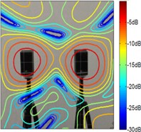
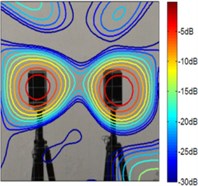
Fig. 4The test results of coherent sources at 1.5 kHz

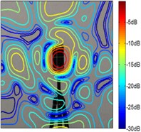
a) CBF

b) Improved FB with $v=$ 1

c) Improved FB with $v=$ 3

d) Improved FB with $v=$ 10

Fig. 5The test results of single monopole at 2.5 kHz

a) CBF

b) Improved FB with $v=$ 1

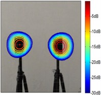
c) Improved FB with $v=$ 3

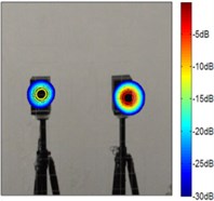
d) Improved FB with $v=$ 10

According to Fig. 4 and Fig. 5, the source maps of conventional beamforming are blurred by the sidelobes and ghost lobes, and it creates a wider beam. However, similar to the simulation results, whatever sources the sound maps estimated by the improved functional beamforming with a larger order $v$ are better to locate the source. It highlight that the improved method can eliminate sidelobes and increasing the spatial resolution.

Results obtained by the proposed beamforming method with “virtual array” show a series of advantages compared to using conventional beamforming. Firstly, the cost of four microphones compared with 36 microphones which has been reduced is a huge difference. Also, due to the improved functional beamforming with a high resolution, the flexibility of the proposed method allows to be easily used in source localization.

5. Conclusions

A new source localization method called improved functional beamforming using a virtual array has been developed to improve the dynamic rage and the resolution of the beamforming method. By combining functional beamforming and virtual array, the proposed method has is able to capture the source locations with substantial increasing in dynamic rage. The proposed method has been applied to numerical and experimental tests including single monopole and coherent sources. All results indicate that the proposed method with a larger order $v$ is able to localize source positions with a high resolution.

References

-
Maynard J. D., Williams E.G., Lee Y. Nearfield acoustic holography: 1. Theory of generalized holography and the development of NAH. Journal of the Acoustical Society of America, Vol. 78, Issue 4, 1984, p. 1395-1412.
Veronesi W. A., Maynard J. D. Nearfield acoustic holography (NAH): 2. Holographic reconstruction algorithms and computer implementation. Journal of the Acoustical Society of America, Vol. 81, Issue 5, 1987, p. 1307-1321.
Hald J. Combined NAH and beamforming using the same microphone array. Journal of Sound and Vibration, Vol. 38, Issue 12, 2004, p. 18-25.
Suzuki T., Camier C., Pasco Y., et al. L1 generalized inverse beamforming algorithm resolving coherent/incoherent, distributed and multipole sources. Journal of Sound and Vibration, Vol. 330, Issue 24, 2011, p. 5835-5851.
Brooks T. F., Humphreys W. M. A deconvolution approach for the mapping of acoustic sources (DAMAS) determined from phased microphone arrays. Journal of Sound and Vibration, Vol. 394, Issues 4-5, 2006, p. 856-879.
Comesana D. F., Wind J., Grosso A., et al. Far field source localization using two transducers: a ‘virtual array’ approach. The 18th International Congress on Sound and Vibration Conference, Rio De Janeiro, Brazil, 2011.
Comesana D. F., Holland K., Wind J., et al. Adapting beamforming techniques for virtual sensor arrays. The 4th Berlin Beamforming Conference, Berlin, Germany, 2012.
Dougherty R. P. Functional beamforming. The 5th Berlin Beamforming Conference, Berlin, Germany, 2014.
Dougherty R. P. Functional beamforming for aeroacoustic source distributions. The 20th AIAA/CEAS Aeroacoustics Conference, Atlanta, USA, 2014.
About this article