Abstract
Numerical studies were carried out to investigate the vibration of buried pipeline subjected to blast seismic waves. The numerical model contains a 5 tons of explosive, an X70 buried pipeline and different kinds of soils. The stress and the vibration velocity of the pipeline were acquired during the simulation. The influence of buried depth on vibration velocity was also revealed in the paper.
1. Introduction
Buried pipelines are mainly used for distribution of water, gas, oil, etc., and are considered as the most important elements of lifelines. When subjected to blast seismic wave, the structure may cause serve disasters [1, 2]. Accordingly, analysis of buried pipeline subjected to dynamic loads is popular in recent years.
Newmark [3] and Kuesel [4] first attempt to seismic design of buried pipelines likely be damaged by earthquakes or far explosions. Malachowski et al. [5] applied the blast load to the pipes with and without protective cover using ALE method. Mokhtari [6] used a combined Eulerian-Lagrangian method to study the response of buried steel pipelines to explosion, and generally concerns finding safe distance of explosion where pipeline does not undergo plastic deformation. There are many others use the finite element method, the finite-difference method or their combination to solve the problem [7, 8].
The present paper investigated the dynamic response of buried pipeline subjected to blast wave numerically. An Arbitrary Lagrangian-Eulerian method was adopted to develop a full-coupled 3D finite element model. By choosing proper material models, the dynamic process was studied with accuracy. The velocity and the stress of the pipeline was obtained, and the influence of buried depth was studied in the analysis. The results obtained from the present study can be used for improvement in protective design of steel pipelines.
2. Numerical simulation
2.1. Finite element model
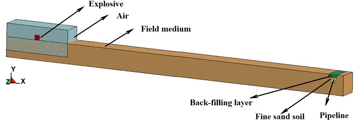
In the present paper, the mechanical performance of buried pipelines subjected to blast wave is studied numerically using nonlinear finite element code LS-DYNA. Considering the symmetries of the geometrical model, to save computation time, a half of the system was modeled as shown in Fig. 1. The ALE model involves six different material types. Eulerian meshes were generated for the explosive and the air. On the other hand, the Lagrangian meshes were used to model the field medium, the back-filling layer, the fine sand soil and buried pipelines. The model was constructed with Solid 164 solid element and g-cm-us unit. The material of the pipeline is X70, with a diameter 1219 mm and wall thickness 26.4 mm. The explosive used in the analysis was emulsion explosive. The distance between the pipeline and the explosion center was around 50 m. The finite element model is shown in Fig. 1.
Fig. 1Finite element model
2.2. Material behavior
The explosive charge was modeled using the high explosive burn material model and the Jones-Wilkin-Lee (JWL) equation of state (EOS). The JWL equation of state defines the pressure as a function of the relative volume, and initial energy per volume, , such that:
where , , , and are material constants, is the pressure, is the relative volume of detonation product and is the specific energy with an initial value of . The emulsion explosive C-J parameters and the JWL equation of state parameters: 0.6 g/cm3, 6.93 km/s, 1.5 GPa, 132.8 GPa, 0.439 GPa, 5.3, 1.2, 0.21, 3.2×10⁹ J/m3, respectively.
Material Type 9 of LS-DYNA (*MAT_NULL) is used to model the behavior of the air. Air mass density and initial internal energy are 1.29 kg/m3 and 0.25 J/cm3, respectively.
There are three different kinds of soils used in the analysis. In order to simulate the behavior of soil in this research, a plastic hardening model was used based on the soil properties. The yield stress and the strain rate has the following relationship:
where , are the Cowper-Symonds strain rate parameters, respectively; is Young modulus; is the initial yield stress; is applied strain rates; is the plastic hardening modulus. The parameters of the model can be seen in [8].
The X70 pipeline material has been modeled using the Johnson-Cook (JC) constitutive relation and the Gruneisen equation of state. The JC model accounts for isotropic hardening, strain rate sensitivity and thermal softening. The model defines the yield stress as:
where , , , and are the material parameters determined by experiments. is the dimensionless effective strain rate for and is the homologous temperature. The parameters of the X70 pipeline can be seen in [9].
2.3. Finite element formation
The damage of the buried pipeline depends mostly upon the stress state. So the analysis of stress distribution can be helpful to the vibration analysis. The wave propagation progress and vibration of the pipeline are studied through numerical simulation.
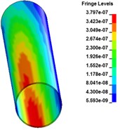
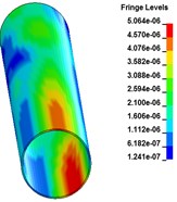
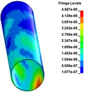
Fig. 4 shows the stress distribution of buried pipeline at different times after explosion. From the figure we can see, the blast waves arrive to buried pipeline at 3.3 ms. Then shock waves propagate to the end side of the pipeline. At the time 11.9 ms, the stress waves travel through the entire pipeline. At this time, the bottom earth generates a resistance to prevent the vibration of the pipeline and produce the stress concentration at the bottom face of the pipeline. With the vibration of the pipeline, the stress concentration area keeps decreasing. At 70 ms, there is little stress left on the surface of the pipeline.
Fig. 2Stress distribution of buried pipeline at different times

a) 3.3 ms
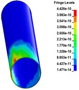
b) 8.4 ms
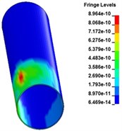
c) 9.4 ms
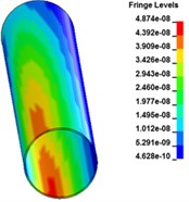
d) 11.9 ms
e) 12.3 ms
f) 14.8 ms
g) 30 ms
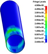
h) 70 ms
3. Results and discussion
3.1. Velocity analysis
After explosion, the middle points of the pipeline are closest to the explosion center. The vibration of the middle points of the pipeline need to be observed intensively. So we choose four points on fracture surface, namely A, B, C and D to analysis the vibration. The positions of the points are shown in Fig. 3. The velocity of the four points are analyzed.
Fig. 3The cross section of the pipeline
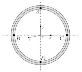
Fig. 4 shows the velocity-time curves of the four points at the cross section. The distance from the explosion center is 50 m, and the buried depth 1.2 m. From the figures we can see, when the stress wave propagates to point A, the body wave contribution most to the vibration velocity in the direction and direction. The amplitude and scope are almost the same in the two directions. The peak velocities of point A and B are 1.17 cm/s and 1.98 cm/s in the reverse direction. The vibration velocity in the direction is small and can be ignored. On the other hand, the peak velocities of point C and D are 0.69 cm/s and 2.13 cm/s in the reverse y direction. The velocity in the direction can also be ignored.
Fig. 4Velocity-time curves of the points at the cross section
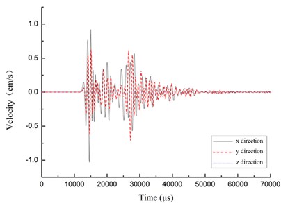
a) Point A
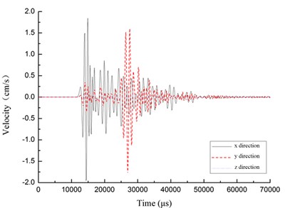
b) Point B
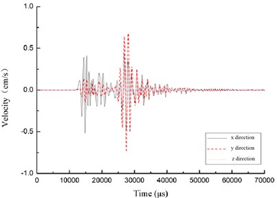
c) Point C
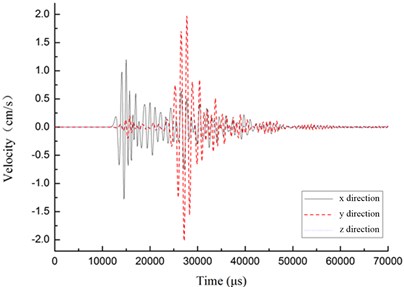
d) Point D
Fig. 5Peak velocity curves in radial direction
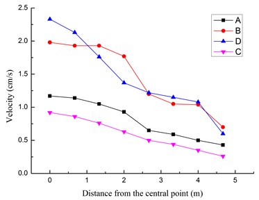
Fig. 6Peak velocity curves in circumferential direction
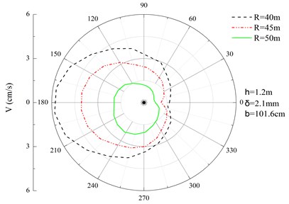
Fig. 5 shows the radial peak velocity curves of four points. The figure shows that with the increase of the distance to the end of the pipeline, the peak velocity keeps decreasing. At the distance of 4.7 m from the central point, point C has the smallest velocity 0.26 cm/s of the four points, while point B and D have almost the same velocity values. Fig. 6 shows the distribution of peak velocity in circumferential direction at the cross section. From the figure we can see, with the increase of the distance from the explosion center, the peak velocity shows downtrend. The largest velocity appears at the left side of the pipeline and the smallest velocity appears at the right side.
3.2. Influence of buried depth
Figs. 7-9 show the peak velocity curves at the middle point of the pipelines with the distance from the explosion center 45 m, 50 m and 60 m, respectively. From the figures we can see that circumferential vibration velocity increase with the increase of buried depth. The differences of the peak velocities among different depth decrease with the increase of the explosion distance. At the distance of 60 m, the peak velocities among different depth become almost the same.
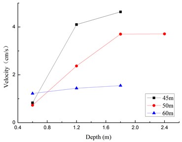
Fig. 10 shows the relationship between circumferential vibration velocity and the buried depth. From the figure we can see that the vibration velocity decrease with the increase of the distance from the explosion center. At the buried depth of 0.6 m, the peak velocity change little with the increase of the depth.
Fig. 7Peak velocity curves at the distance of 45 m
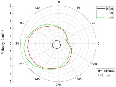
Fig. 8Peak velocity curves at the distance of 50 m
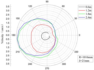
Fig. 9Peak velocity curves at the distance of 60 m
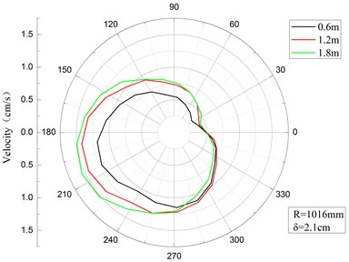
Fig. 10Relationship between peak velocity curves and buried depth
4. Conclusions
The vibration of the buried pipeline was studied numerically in the paper. The stress and the vibration velocity were studied through numerical simulation. The influence of buried depth was also acquired. The results show that, with the decrease of the distance to the end of the pipeline, the radial peak velocity becomes smaller, and with the increase of the distance from the explosion center, the peak velocity shows downtrend. The circumferential vibration velocity increases with the increase of buried depth, and at the buried depth of 0.6 m, the peak velocity change little with the increase of the depth.
References
-
Isoyama R., Katayama T. Practical performance evaluation of water supply networks during seismic disaster, lifeline earthquake engineering. The Current State of Knowledge, ASCE, 1981, p. 111-122.
-
Toki K., Sato T. Estimation of damage of water distribution systems by earthquakes. Recent Advance in Lifeline Earthquake Engineering in Japan, ASME, 1985, p. 89-96.
-
Newmark N. M. Problems in wave propagation in soil and rock. Proceedings of International Symposium on Wave Propagation and Dynamic Properties of Earth Materials, University of New Mexico Press, Albuquerque, 1968, p. 7-26.
-
Kuesel T. R. Earthquake design criteria for subways. Journal of the Structural Division, 1969, p. 1213-1231.
-
Malachowski J., Mazurkiewicz L., Gieleta R. Analysis of structural element with and without protective cover under impulse load. Proceedings of 12th Pan-American Congress of Applied Mechanics, Port of Spain, Trinidad, 2012.
-
Mokhtari M., Alavi Nia A. A parametric study on the mechanical performance of buried X65 steel pipelines under subsurface detonation. Archives of Civil and Mechanical Engineering, Vol. 15, 2015, p. 668-679.
-
O’Daniel J. L., Krauthammer T. Assessment of numerical simulation capabilities for medium-structure interaction systems under explosive loads. Computers and Structures, Vol. 63, 1997, p. 875-887.
-
Lu Yong, Wang Zhongqi, Chong Karen A comparative study of buried structure in soil subjected to blast load using 2D and 3D numerical simulations. Soil Dynamics and Earthquake Engineering, Vol. 25, 2005, p. 275-288.
-
Ji Chong, Long Yuan Local damage effects of X70 steel pipe subjected to contact explosion loading. Chinese Journal of High Pressure Physics, Vol. 27, 2013, p. 567-574
About this article

This research was financially supported by the National Nature Science Foundation of China, No. 11102233. The authors would like to gratefully acknowledge this support.
