Modeling and control of a demonstrative prototype for platform multi-launcher rocket system using Lagrange’s equation and CATIA simulation

1. Introduction

This paper will describes research and development a demonstrative prototype for platform of Multi-Launcher Rocket System (MLRS) at laboratory in Defence Technology Institute of Thailand. In order to design the controller for any dynamical system, a suitable dynamical model of the system needs to be formulated and its parameters need to be accurately identified. The Important parameters were obtained with various methods. Some parameters were obtained research and developed, manufacturer specifications, and some parameters needed to be obtained through experiments and test. This also holds for a demonstrative prototype for platform of Multi-Launcher Rocket System (MLRS), this paper proposes the system identification using Lagrange’s equation and control simulation analysis tool were identified and the model was developed, then the model was employed to simulate the multi-sine input signal and the simulation results were compared to the experimental results for validation the model. This paper was organized in the following manner: Section 2 – plant; Section 3 – modeling of the plant; Section 4 – root locus and stability analysis; Section 5 – controller design; Section 6 – experimental results and discussion; finally, Section 7 is the conclusion.

2. Plant

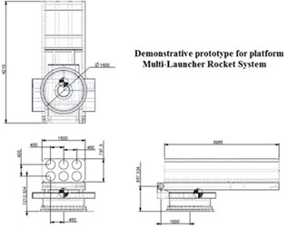
The plant used of this research is the demonstrative prototype for platform of MLRS as shown in Fig. 1. The platform consists of three major parts as following: 1) The turning use for construction of azimuth angle parts that has diameter 1600 mm height 637 mm in width length and thickness respectively and the total weight is 2,879 kg; 2) The cradle use for construction of elevation angle platform is the all of the elevation control devices and rocket pod that has dimension 1,500 mm 4,210 mm and 250 mm in width, length and thickness respectively and the total of weight is 928 kg; 3) The rocket pod include launch tube 6 tube that has dimension 1,500 mm, 3,965 mm, 797 mm and the total weight 838 kg. The pressurized fluid flow is controlled by using the programmable logic controller. This control solenoid valve is the proportional and directional type that have analog input voltage 0-10 VDC with current 0-20 mA. The hydraulic drive system is driven by the user pressurized pump and solenoid valve are regulate fluid source of up to 2200 psi or 150 bars. The Also this research studies together with CATIA V6 simulation to simulate and determine the parameters use for Lagrange’s equation as shown in Fig. 1.

Fig. 1Dimension of demonstrative prototype for platform multi-launcher rocket system

3. Modeling of the plant

3.2. Lagrange’s equation for the azimuth angle control

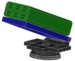
The model of the azimuth angle control of a demonstrative prototype for platform of MLRS can be written by Lagrange’s equation and determine the parameters of the plant using CATIA V6 simulation as shown in Fig. 2.

Fig. 23D simulation of the azimuth angle control

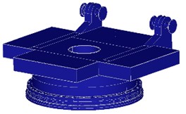
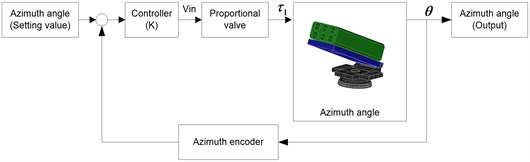
Fig. 3Block diagram of the azimuth angle control

The parameters of the azimuth angle control system that difficult to determine the actually value. This research presents the method using CATIA V6 simulation to determine the center of gravity ($CG$), length of $CG$ to joint ($l$), mass ($m$), gravitational ($g$), and inertia ($J$) respectively. The results as shown in Table 1.

Table 1Parameters of the azimuth angle control system

Parameters	Result	Unit
Center of gravity on $x$-axis ($C{G}_x$)	142.52	mm
Center of gravity on $y$-axis ($C{G}_y$)	643.43	mm
Center of gravity on $z$-axis ($C{G}_z$)	246.86	mm
Length of $CG$ to joint ($l$)	98.58	mm
Mass ($m$)	2,879	kg
Inertia ($J$)	1,543.08	kg/m2
Gravitational ($g$)	9.81	m/s2

2

$J\ddot{\theta }+mgl\mathrm{s}\mathrm{i}\mathrm{n}\theta =r{\tau }_l,$

3

$\mathrm{1,543.08}\ddot{\theta }+\left(\mathrm{2,879}*9.81*0.098\right)\mathrm{s}\mathrm{i}\mathrm{n}\theta ={\tau }_1,$

4

$\mathrm{1,543.08}\ddot{\theta }+\mathrm{2,767.81}\mathrm{s}\mathrm{i}\mathrm{n}\theta ={\tau }_1.$

Eq. (4) is a non-linear equation. This research was considered in the range of operating and linearized [10] by $\mathrm{s}\mathrm{i}\mathrm{n}\theta \approx \theta$. Thus:

5

$\mathrm{1,543.08}\ddot{\theta }+\mathrm{2,767.81}\theta ={\tau }_1.$

Then, take Laplace transform and determine the transfer function of azimuth plant as following:

6

$\mathrm{1,543.08}{s}^2\theta \left(s\right)+\mathrm{2,767.81}\theta \left(s\right)={\tau }_1\left(s\right),$

7

$G_1\left(s\right)=\frac{\theta \left(s\right)}{{\tau }_1\left(s\right)}=\frac{1}{\mathrm{1,543.08}{s}^2+\mathrm{2,767.81}}.$

From Eq. (7) is the open-loop azimuth angle plant, but the real demonstrative prototype for platform of multi-launcher rocket system using PLC and the hydraulic drive system is driven by METARIS pump hydraulic model MHP350B478 with the maximum flow 200 L/min and HAWE proportional valve with input signal ±10 Vdc, the maximum flow 200 L/min at pressure 200 bar, the maximum torque 350 Nm as shown the block diagram of the azimuth angle control in Fig. 3. Thus, determine the transfer function of the azimuth angle control with the output has a unit in degree as below:

8

$G_{azi}\left(s\right)=\frac{\theta \left(s\right)}{V_{in}\left(s\right)}=\left(35\right)\frac{1}{\mathrm{1,543.08}{s}^2+\mathrm{2,767.81}}\left(\frac{180}{\pi }\right),$

9

$G_{azi}\left(s\right)=\frac{\theta \left(s\right)}{V_{in}\left(s\right)}=\frac{1.29}{s^2+1.79}.$

3.3. Lagrange’s equation for the elevation angle control

The model of the elevation control system of the demonstrative prototype for platform of MLRS can be written as Lagrange’s equation and determined the parameters by CATIA V6 simulation as shown in Fig. 4.

From the result CATIA V6 simulation to determine the parameters of the elevation angle control to determine the center of gravity ($CG$), the length of $CG$ to joint ($l$), mass ($m$), gravitational ($g$), and inertia ($J$) respectively that the results as shown in Table 2.

10

$J\ddot{\varphi }+mgl\mathrm{s}\mathrm{i}\mathrm{n}\varphi ={\tau }_2,$

11

$\mathrm{2,173.19}\ddot{\varphi }+\left(\mathrm{3,328.54}*9.81*0.870\right)\mathrm{s}\mathrm{i}\mathrm{n}\varphi ={\tau }_2,$

12

$\mathrm{2,173.19}\ddot{\varphi }+\mathrm{28,403.48}\mathrm{s}\mathrm{i}\mathrm{n}\varphi ={\tau }_2.$

Table 2Parameters of elevation angle control system

Parameters	Result	Unit
Center of gravity on $x$-axis ($C{G}_x$)	90.15	mm
Center of gravity on $y$-axis ($C{G}_y$)	1,241.53	mm
Center of gravity on $z$-axis ($C{G}_z$)	156.15	mm
Length of $CG$ to joint ($l$)	870	mm
Mass ($m$)	3,328.54	kg
Inertia ($J$)	2,173.19	kg/m2
Gravitational ($g$)	9.81	m/s2

Eq. (12) is a non-linear equation. This research was considered in the range of operating and linearized [10] by $\mathrm{s}\mathrm{i}\mathrm{n}\varphi \approx \varphi$. Thus:

13

$\mathrm{2,173.19}\ddot{\varphi }+\mathrm{28,403.48}\varphi ={\tau }_2.$

Then, take Laplace transform and determine the transfer function of elevation plant as following:

14

$\mathrm{2,173.19}{s}^2\varphi \left(s\right)+\mathrm{28,403.48}\varphi \left(s\right)={\tau }_2\left(s\right),$

15

$G_2\left(s\right)=\frac{\varphi \left(s\right)}{{\tau }_2\left(s\right)}=\frac{1}{\mathrm{2,173.19}{s}^2+\mathrm{28,403.48}}.$

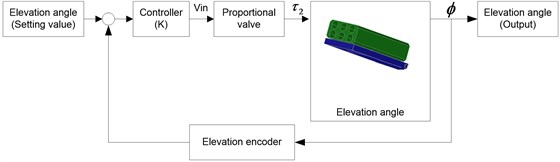
From Eq. (15) is the open-loop elevation angle plant, but the real demonstrative prototype for platform of multi-launcher rocket system using PLC and the hydraulic drive system is driven by METARIS pump hydraulic model MHP350B478 with the maximum flow 200 L/min and HAWE proportional valve with input signal ±10 Vdc, the maximum flow 200 L/min at pressure 200 bar, the maximum torque 350 Nm as shown the block diagram of the elevation angle control in Fig. 5. Thus, determine the transfer function of the closed-loop control for elevation angle control with the output has a unit in degree as below:

16

$G_{ele}\left(s\right)=\frac{\varphi \left(s\right)}{V_{in}\left(s\right)}=\left(35\right)\frac{1}{\mathrm{2,173.19}{s}^2+\mathrm{28,403.48}}\left(\frac{180}{\pi }\right),$

17

$G_{ele}\left(s\right)=\frac{\varphi \left(s\right)}{V_{in}\left(s\right)}=\frac{0.92}{s^2+13.07}.$

Fig. 43D simulation of the elevation angle control

Fig. 5Block diagram of the elevation angle control

4. Root locus and stability analysis

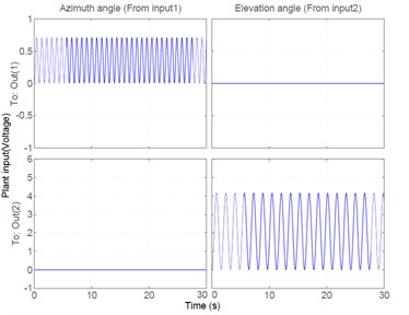
From the state space model can analyze the root locus of the plant found that the azimuth angle control systems has poles at ±1.3379i on the imaginary axis and the elevation angle control system has poles at ±3.6152i on the imaginary axis as shown in Fig. 4. Thus the system of a half-scale of MLRS is an unstable open loop plant. The state space model can analyze stability using a unit step input to determine the step response of the open loop system, the result shown as Fig. 5 that consists of output1: Azimuth angle (From input1) and output2: Elevation angle (From input2) and the results of step response of open loop system is an unstable system. Therefore, the system of a half-scale of MLRS is an unstable open loop plant.

Fig. 6Root locus of the open loop plant

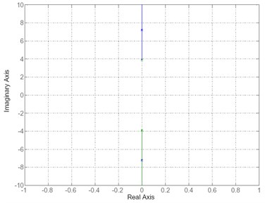
Fig. 7Step response of the open loop system

5. Controller design

The plant of a demonstrative prototype platform for multi-launcher system was the unstable open loop plant. Then the pole-placement method [8, 9] was used for the design of feedback controller as block diagram in Fig. 6 and Fig. 7. This method enables all poles of the closed-loop to be placed at desired location and providing satisfactory and stable output performance. Thus the closed-loop plant of the azimuth angle control has a new pole at –0.25±0.3766i and the elevation angle control has pole at –0.3637±0.5478i as shown in Fig. 8.

6. Experimental results and discussion

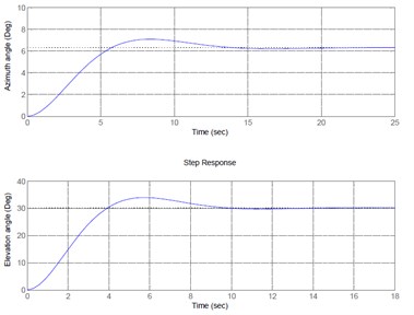
The comparison of the experimental results and simulation results of the model using Lagrange’s equation that excited by multi-sine input signals found that the model using Lagrange’s equation of azimuth angle control having percentage best fit of 92.24 % and the model of elevation angle control having percentage best fit of 90.13 % respectively. And the step response of the closed-loop plant have improved and met the requirement as shown in Fig. 9.

Fig. 8Root locus of the closed-loop plant

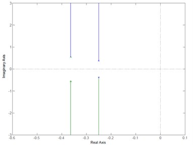
Fig. 9Step response of the closed-loop plant

7. Conclusion

The modeling of a demonstrative prototype for platform of MLRS using Lagrange’s equation and CATIA simulation were identified, then the model was employed to simulate the multi-sine input response and the simulation results were compared to the experimental results. It was found that the model can be accepted and meet to the requirements.

The simulation and experimental results are given small differences. This is due to the abilities of electronic valve to open and close at its capabilities rate. Further investigations have to be conducted to explain and improve the accuracy of the model.