Abstract
The vibrations of pantograph passing underneath the overhead system can be reduced by using droppers to place the contact wire in the designed curve. Nowadays, various software programs are used to estimate dynamic interaction of pantographs and overhead catenary system. In order to implement the software program, the necessary static force for each dropper should be estimated initially to place the contact wire in the designed curve. Unlike most available software programs, the implemented software program in this research consists of a heuristic analytical algorithm to estimate the static shape of the overhead catenary system. Accordingly, the variable separation and eigen function expansion method were used to calculate the static shape of contact wire and messenger cable under a given loading condition. At the next step, the stiffness matrix of contact wire in catenary was obtained and a procedure was defined to calculate the necessary static force for each dropper, which would then place the contact wire in the target curve. Finally, effort was made to examine the function of automatic tension device in OCS (Tension Wheel considering the Coulomb’s friction). Moreover, the deformations in the contact wire and messenger cable due to temperature changes were estimated and the results shows that allowable friction in the tension wheel can cause 27 % deviation in sag of the contact wire.
1. Introduction
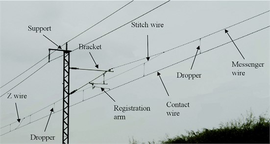
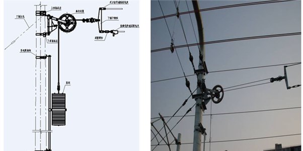
The electrification of a fleet normally involves either a third rail or an overhead catenary system. Since the high-speed fleets use only overhead catenary systems, numerous studies have focused on dynamic interaction of high speed pantograph and overhead catenary system. Fig. 1 illustrates the overhead system and its components [1].
Fig. 1Overview of the components of overhead system
Generally, previous studies focused on the dynamics of pantograph and overhead catenary system to maintain the connection between pantograph and contact wire at higher speeds. The fluctuations of contact force have been examined as the main factor threatening the permanent contact between pantograph and contact wire. In fact, effort has been made to minimize such fluctuations through optimization of the elements used in the pantograph or catenary system. A multitude of software programs written in this field in recent years reflects the importance of the issue [2-11]. In addition, part of the researches are concentrated with controlling the pantograph through the estimation of the level of force via various methods and prevent any significant changes by applying controlling forces [12-14]. There are limited analytical studies as compared to those focusing on the finite element method. However, certain studies have examined the issue through dynamic wave propagation in catenary system or even a tensioned beam [15, 16]. Each software developed to study the dynamics of pantograph and catenary system can calculate through different procedures and accuracies the initial conditions of the overhead catenary system. Despite the plurality of such studies, there is still some uncertainty about the initial shape and static force of the overhead system [17]. Some studies have explored only the method of obtaining initial conditions of overhead systems [1]. In this study, the contact and messenger cables with a tensioned Euler-Bernoulli beam were modeled. Then, the variable separation method has been used to obtain the natural frequencies and mode shapes of the contact wire and the messenger cable individually. At the next step, eigenfunctions expansion has been used to obtain the static shape of wire under each loading case. A unit force at the location of droppers has been applied to obtain the stiffness matrix of contact wire. Then, the static forces of droppers were calculated to achieve any given curve of the contact wire. These values were compared against the results of other software programs around the world. The acceptance criteria of tension wheel performance test were employed to estimate the level of deformations in the contact wire and messenger cable under an automatic tension device. Accordingly, the value of allowable tension deviation for a tension wheel was considered as the tension forces were applied to the contact wire and messenger cable once at the upper limit and once at the lower limit, so as to calculate the variations in deflection of sag of contact wire due to temperature fluctuations.
2. Problem statement
As noted earlier, this problem can be solved through finding out a set of forces (as the dropper’s deal load or static force) applied on certain points of the tensile beam (as the contact wire) in order to place the contact wire in particular shape (as the target curve). In the other words, the equilibrium shape of contact wire due to its own weights and set of dropper’s forces, needs to be as much as possible approximate to the target curve. Target curve of contact wire can be supposed as a horizontal line (0) or with small down ward pre-sag.
Fig. 2Problem definition. gray line: Contact wire influenced by its own weight, dotted line: Target curve for the contact wire, solid black line: Contact wire after applying appropriate set of forces at dropper location points, Red Arrows: Calculated dropper forces
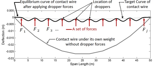
The problem is depicted in Fig. 2 and as it can be seen, the gray line indicates the contact wire shape under its own weight, while the dotted line has displayed the target curve or desired shape of contact wire. If the concentrated forces exerted by the droppers on the contact wire (red arrows) are selected correctly (the values of calculated forces for this example are presented in Table 1), the curve shown in solid black curve can be achieved. In solid black curve, both the forces of gravity as well as droppers influence the wire. The distance between red arrows in Fig. 2 are equal to the distance between droppers in catenary. Table 2 shows the specifications of the beam as contact wire and messenger cable. For example, if the deflection objective function is the parabola mentioned in [18], it needs to be applied onto the wire at 10 points of the forces displayed in Table 1 so that the wire can be placed precisely on the deflection objective function at points where the force is exerted.
Later in this study, the path required to obtain these forces will be explored.
Table 1Position of the droppers in each span (measured from the left end of the span) and pre-sag prescribed for the contact wire at the droppers and required static force for each dropper
Position (m) | 5 | 10 | 15 | 20 | 25 | 30 | 35 | 40 | 45 | 50 |
Target curve (mm) | 0 | 24 | 41 | 52 | 55 | 55 | 52 | 41 | 24 | 0 |
Force value (N) | 192.06 | 51.30 | 53.88 | 49.19 | 53.93 | 53.93 | 49.19 | 53.88 | 51.30 | 192.06 |
3. Modeling of the problem
Due to the significant value of tension in the catenary system, a tensile Euler- Bernoulli beam has been considered as a wire model. Moreover, as the wire showed a significant amount of bending resistance at the points where the forces are applied, the string model could not be adopted. Eq. (1) formulates the governing differential equation for transverse displacement in the tensile beam:
In Eq. (1), is the beam’s transverse displacement in time and space , is the mass per unit length of wire, is the beam’s damping coefficient, is the axial load applied to the beam ( is positive in tension), and is the beam’s bending stiffness. The gravity load () and the concentrate force exerted by droppers () are also involved on the right side of the Eq. (1). Although this is a static problem where the variations are Meaningless over time, there are two reasons why the dynamic differential Eq. over the tensile beam and the governing procedures is used to solve this problem. Firstly, this is generally a pre-processing problem to obtain the dynamic response of the catenary system from the passing pantograph. Hence, the modal analysis of the beam needed to be done in each case. It is better to clarify the initial conditions through coefficients of eigenfunctions based on Rrighly-Ritz quotenet. Secondly, mode shapes of the wire, either higher or lower, could be selected depending on the precision required. That is why the initial conditions must have the capability to be described through higher or lower number of mode shapes.
Eq. (2) formulates the boundary and initial conditions:
Relying on the separation of variables, the solution can be formulated in two separate sections as . Then by inserting Eq. (2) into the homogeneous part of Eq. (1), Eq. (3) can be achieved:
The temporal and spatial functions are equal only if they are equal to a constant value (Eq. (4)). According to the differential Eq. (1) governing the temporal section, the square value represents the natural frequency ():
By formulating the differential Eq. (1) governing the spatial section, the spatial functions applying to this differential Eq. (1) can be obtained as illustrated in Eq. (5):
In Eq. (5), represents the spatial section of the response. Similarly, displays the function as a vector which is multiplied by the coefficients vector ( in Eq. (6)) so as to describe the spatial section of the response. Values of and are also functions of placed on the spatial section of the response. Considering the boundary conditions in the solution, the values of and the corresponding mode shape can be obtained. In order to codify Eq. (5), it is better to first define the matrices and as well as vector according to Eq. (6):
In Eq. (6), each column of the matrix is the coefficient of values , , and , respectively. Moreover, each row is the differentiation with respect to time of the previous row by placing 0 or instead of . In matrix the boundary conditions are considered for , while the boundary conditions are included in matrix . Relying on the two matrices as well as the type of both conventional and unconventional boundary conditions (pined heads, fixed heads, elastic support, etc.), coefficient matrix can be attained. Eq. (7) shows how the matrix of coefficients is formulated:
The system of linear Eq. (7) reflecting the boundary conditions is obtained through the product of coefficient matrix () in the coefficient vector (). Since the coefficient vector could not be zero, the determinant of the coefficient matrix should have been zero (Eq. (8)):
As mentioned above, the values of elements in the coefficient matrix are functions of . Hence, leading to zeroed determinant of the coefficient matrix can be found and introduced as natural frequencies. In order to obtain the mode shapes, each of these natural frequencies were inserted into the coefficient matrix. Then, one of the arrays of coefficient vector was set to be 1 so as to achieve the matrix Eq. (9):
where is the number of considered natural frequencies. Eq. (10) shows how the arrays of coefficient vector are obtained to describe the mode shapes:
Eq. (10) shows how the mode shapes corresponding to each natural frequency are described:
The eigenfunction expansion or Galerkin’s method served to convert the partial differential equations (PDEs) to ordinary differential equations (ODEs). In this procedure, it is assumed that the final response of Eq. (1) can be extended through a linear combination of mode shapes multiple a series of temporal coefficients. Hence, the solution can be extended according to Eq. (12):
By inserting the solution in the differential Eq. (1) Eq. (14) can be achieved:
If the two sides of the Eq. (13) is multiplied by (mode shape th) and integrated from zero to , the orthogonality of mode shapes can be employed, since the conventional boundary conditions are supposed:
Finally, integrating and orthogonal shape modes are employed to obtain the ordinary differential Eq. (15):
As mentioned earlier, the objective is to find the static deflection of equilibrium state of wire under various loads such as gravity or dropper force. In this scenario, the wire is stationary, which is why the first and second temporal differentiation in Eq. (15) can be zeroed to formulate the linear Eq. (16):
By Eq. (16), the coefficients of each mode shape can be achieved and then the shape of wire can be obtained through their linear product to the mode shape vector.
Afterwards, if single unit of force is applied at , then the corresponding displacement at point can be displayed through , as shown in Fig. 3.
If the unit loads are exerted at the location of droppers and the measurements are also at the place of droppers, then the stiffness matrix of contact wire can be formulated in accordance with Eq. (17):
Fig. 3Definition of elements of stiffness matrix in the overhead system (in two different loading points)
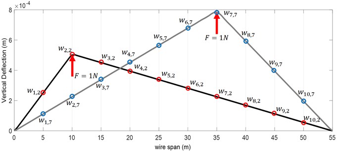
In Eq. (17), order to deflection of the junction of the second dropper under the unit load at the junction of the third dropper. Moreover, shows the number of droppers.
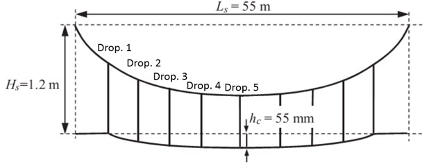
The purpose of using droppers is to remove the normal sag of contact wire and to shape it to an approximate certain target curve. The droppers will apply the most optimum static force to the contact wire when the junction between the dropper and the contact wire is placed at the target curve. The target curve can also be expressed both as a function and as a vector indicating the favorable points of contact wire at the junction of droppers (as it is presented in Table 1). In some case the target curve of contact wire is presented only by mid-span deflection of contact wire (For example 55 mm) in Fig. 4. In such case the Eq. (17) of target cure can be considered as a fitted curve on points (0,0), (,) and (, 0). The coefficients of target curve can be extracted by any curve fitting approach. Eq. (18) shows an example of function of target curve:
Therefore, the junction between each dropper and the contact wire should reach the corresponding point on the target curve. Without involvement of droppers, the wire would be subject to its weight as a function of . Hence, the displacement provided by the th dropper at the junction would be equal to: . By considering stiffness matrix of the contact wire, Eq. (19) can be used to estimate the static force of each dropper:
Hence, the static force of droppers can be calculated with regard to the limited number of mode shapes in order to achieving the target curve.
4. Results and discussion
The first step is to verify the authenticity of obtained forces, the value and location of forces are inserted in Eq. (16) to obtain the static deflection of wire under the sum of static forces of droppers and its weight. Similarly, the reaction of these forces are exerted on the messenger cable so as obtain its shape. Fig. 4 shows the geometry of span under study and the values in Table 2 and Table 3 are used to achieve the results of this study [18].
Fig. 5 illustrates an overview of static deflection obtained for the contact wire and the messenger cable under calculated forces.
Fig. 4The overhead system model and geometrical data applied
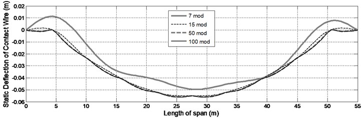
As seen in the Fig. 5, the estimated static force can sufficiently render the junction of droppers at the target curve. In order to evaluate the contribution of mode shapes, the problem was solved four times, where 7, 15, 50 and 100 first mode shapes were considered, respectively. The results have been displayed in Fig. 6.
Fig. 5Overview of calculated static mode for the overhead system
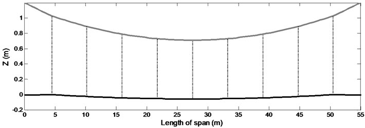
Table 2The assumed values for the contact wire and messenger cable so as to achieve the results
The geometric data of the span | Sectional data of the contact wire | Sectional data of the messenger wire | |||
Span length | 55 m | Section, Ac | 150 mm2 | Section, Am | 120 mm2 |
Encumbrance | 1.2 m | Mass/unit length, mc | 1.35 kg/m | Mass/unit length, mm | 1.08 kg/m |
Pre-sag at mid-span, hc | 55 mm | Tension, Sc | 22kN | Tension, Sm | 16 kN |
Stagger | ±200 mm | Young’s module, Ec | 1.0e11N/m2 | Young’s module, Em | 0.97e11 N/m2 |
Bending stiffness, EcJc | 195.0 N m2 | Bending stiffness, EmJm | 131.7 N m2 | ||
Table 3The optimal position of droppers and points for suitable junction between droppers and contact wire
Dropper | 1 | 2 | 3 | 4 | 5 | 6 | 7 | 8 | 9 |
Position (m) | 4.50 | 10.25 | 16.00 | 21.75 | 27.50 | 33.25 | 39.00 | 44.75 | 50.50 |
Sag (mm) | 0 | 24 | 41 | 52 | 55 | 52 | 41 | 24 | 0 |
Fig. 6 suggests that the accuracy of results can be enhanced through considering a specific number of mode shapes so that at highest natural frequency (and according to its corresponding mode shape), there is always at least one antinode forming between two adjacent droppers. In other words, the mode shape concerning the highest considered natural frequency should form one antinode between two adjacent droppers or the smallest considered wave length, should be smaller than distance between three adjacent droppers. In addition, if more frequencies are considered, there will be no significant increase in the accuracy of results, i.e. only the volume of calculation would increase.
Fig. 6The effect of increasing the number of mode shapes on increased accuracy of calculation for static shape of contact wire
4.1. Validation of results
In 2014, [18] introduced a reference model where the certain parameters were given to 10 research companies operating in dynamics of the pantograph and the overhead system. Finally, the solutions were compared to achieve a highly suitable reference for comparing other related studies. In the comparison section, the results of dynamics concerning the passage of pantograph underneath the catenary system and the static parameters of overhead system have been reported. For example, Table 4 displays the static forces obtained through each of these software programs for droppers and then they were compared against the static forces involved in the current study (named CatAna).
Table 4Comparison between the static forces of droppers in various FEM or FDM software programs and analytical solution by this study
SW name | Drop. 1, 4.50 | Drop. 2, 10.25 | Drop. 3, 16.00 | Drop. 4, 21.75 | Drop. 5, 27.5 | Total force of all droppers | % Error (weight of contact wire) |
PrOSA | – | – | – | – | – | – | – |
PantoCat | 169.45 | 49.14 | 55.44 | 47.38 | 55.42 | 698.24 | -6.16 |
SPOPS | 198.10 | 53.06 | 54.24 | 54.17 | 54.15 | 773.29 | 3.92 |
CaPaSIM | 161.98 | 52.14 | 51.90 | 51.98 | 51.69 | 687.69 | –7.58 |
PCaDA | 195.57 | 52.15 | 52.10 | 52.08 | 52.06 | 755.86 | 1.58 |
Gasen-do | 171.32 | 50.09 | 55.89 | 47.80 | 55.84 | 706.04 | –5.12 |
OSCAR | 167.90 | 50.67 | 55.47 | 47.52 | 55.39 | 698.51 | –6.13 |
PCRUN | 162.61 | 52.43 | 56.20 | 48.55 | 56.20 | 695.78 | –6.49 |
CANDY | 155.56 | 52.24 | 56.58 | 48.01 | 54.80 | 679.58 | –8.67 |
PACDIN | 164.14 | 50.30 | 55.30 | 47.34 | 55.29 | 689.45 | –7.35 |
CatAna | 192.06 | 51.30 | 53.88 | 49.19 | 53.93 | 761.80 | 0.36 |
By examining diagrams presented in [18], it can be argued that certain software programs considered the end steady arm of contact wire as a low-stiffness spring, where others considered it as a fixed point in the start and end point of span. The code written in the two states were solved and the result were displayed in Fig. 7. Since reference [18] compared more than 10 software programs which estimated the static curve of contact wire very close to each other, all the Fig. ?? were compared together as a level. As illustrated well in the two Fig. ??, the analytical method was adequately consistent in estimating the static state of the contact wire.
Because the droppers are placed in symmetrical layout at the opening, the forces of the four end droppers were equivalent to the four initial droppers. Regarding the static equilibrium of contact wire the weight of which is entirely tolerated by the droppers, the sum of static forces of droppers should either be equal to the weight of wire and its attachments or be slightly deflected from it. The final column of Table 4 displays the deviation of whole dropper forces from the weight of contact wire and it’s Paraphernalia (such as clamp of dropper and steady are) at one span. As can be seen, most related software programs used the finite element or difference method leading to a considerable error, i.e. the sum of forces exerted by the droppers on the wire is not equal to the weight of contact wire and it’s Paraphernalia. However, there is a slight error in the analytical solution in this study. These errors occur mainly because the steady arm conditions are not transparent. As mentioned earlier, several software programs have modeled it as a fixed point, while others involve a low-stiffness spring. Either way, part of the wire’s weight and it’s Paraphernalia are supported by steady arm, thus leading to an error. This error is less likely in the analytical solution. Moreover, such error is curtailed as the mode shapes increase.
4.2. Effect of temperature variations
The sag of contact wire and messenger cable in the overhead system should not be changed due to temperature variations, because it may severely change the contact force as the pantograph passes. Therefore, the overhead system uses an auto tension device. This device can eliminate the temperature-caused expansion and contraction through spring forces or gravity of counter weight. Any automatic tensioning device that uses gravitational force is also called a tension wheel. Fig. 8 illustrates an example of tension wheel as an automatic tensioning device.
Fig. 7Comparison between the results of analytical code and FEM software programs: a) when the steady arm is rigid, b) when the steady arm is flexible
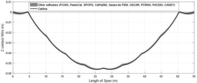
a)
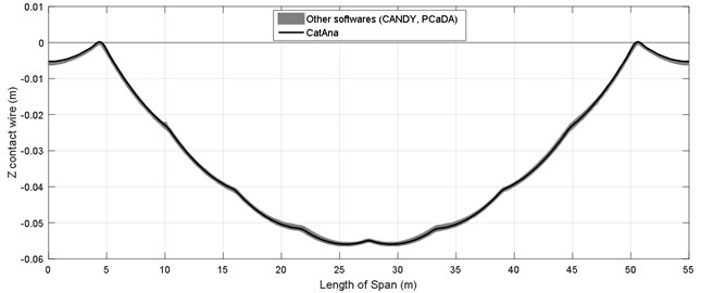
b)
Fig. 8Overview of a tension wheel to maintain tension in the overhead system
Although there is no standard for testing these devices, Siemens conducts three types of tests at the delivery of its parts, the results of which will be reported. The first test checks the mechanical strength, while the second test assesses the anti-fall brake system of weight and the third test involves the wheel’s periodic performance aiming to measure the difference of forces exerted by the device in a state of expansion and contraction. Fig. 9 Displays schematically how the test is conducted.
Fig. 9Overview of how the tension wheel test is conducted
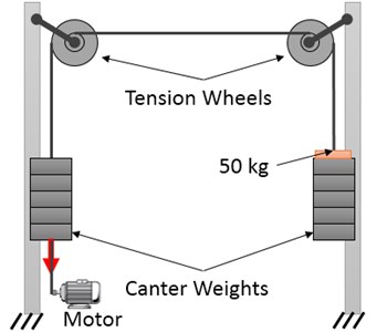
In this test, two tension wheels are placed in front of each other connected by a wire. The identical balance weights are placed on both wheels. In this scenario, the system is in equilibrium and the balance weights can be placed at any height. An additional weight of 50 kg is added to one of the balance weights so as to upset this balance. Moreover, the heavier weights would reach the ground. Afterwards, the lighter weights are dragged down and then released by an electro-motor. The extra 50 kg weight on the other side should overcome the friction of both wheels and pull up the lighter weights. This is repeated 100 times to ensure that the difference in the forces applied during contraction and expansion in the lifetime of wheel will not exceed 490.5 N (50 kg).
Fig. 10Variations of tension force during the circadian rhythm of temperature in the presence or absence of traction wheels
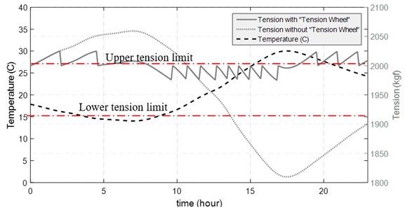
Therefore, it can be assumed that a loaded standard tension wheel can contain the 25 kg of static friction for the wheel to spin (either in clockwise or counterclockwise direction). The Fig. 10 displays the tensions variations in the overhead wire in two scenarios with and without involvement of tension wheels during 24 hours.
The tension force increases as temperature lowers. When tension wheel is involved, the tension will continue rising until its value is lower than the resisting force of static friction at the tension wheel. Then, the weights pull up and prevent further increase in tension. The process also takes place through an increase in temperature. Hence, the tension value of contact force during a day can fluctuate between the upper and lower limits. At the next step, the static mode of contact wire is calculated in the maximum and minimum tension force involved in the wire.
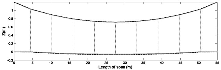
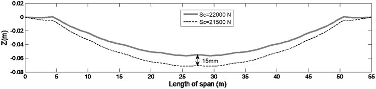
In Fig. 11 based on data in Table 1 and models of overhead systems, the static shape of contact wire and messenger cable under specified tension value and 500 N less than this value, is illustrated.
Fig 11 indicates that the allowable deviation in tension in a standard tension wheel, cause 15 mm (27 %) change at the middle of the sag of contact wire. Moreover, the variations in tension of the messenger cable leads to changes in the sag of the contact wire, whereas variations in the tension of the contact wire lead to change in sag of the sub-spans.
Fig. 11The static deflection charts obtained in high and low tension limits applied by standard tension wheel
a) Whole catenary
b) Contact wire
5. Conclusions
In real catenary installation, the length of droppers is adjusted in a way that contact wire places on target curve of contact wire. But in model of catenary, both analytical and FEM/FDM, dead load of each dropper for placing contact wire in target curve should be calculated. In this study, a new analytical method was presented for calculating the static forces required by droppers in the overhead system through eigenfunction expansion. In continue, it was observed that the estimated forces could adequately approximate the contact wire to the target curve. Furthermore, the values obtained with the static forces for droppers for a particular overhead catenary system have been compared against 10 world-known software programs. It was revealed that the new analytical method was more accurate than other FEM/FDM methods. Therefore, it is recommended that the static forces of droppers in these software program be calculated through an analytical method regarded as initial conditions. Finally, based on the allowable deviation of standard tension wheel in the catenary system, it was found out that if the contact wire and messenger cable are under tension through a standard tension wheel, the variations of sag in contact wire due to temperature variation, will not be over 15 mm. there for it is advised that any dynamic simulation of catenary and pantograph, takes account such deviation in pre-sag of contact wire, especially at higher speed.
References
-
Tur M., et al. A 3D absolute nodal coordinate finite element model to compute the initial configuration of a railway catenary. Engineering Structures, Vol. 71, 2014, p. 234-243.
-
Ambrósio J., et al. PantoCat statement of method. Vehicle System Dynamics, Vol. 53, Issue 3, 2015, p. 314-328.
-
Cho Y. H. SPOPS statement of methods. Vehicle System Dynamics, Vol. 53, Issue 3, 2015, p. 329-340.
-
Collina A., et al. PCaDA statement of methods. Vehicle System Dynamics, Vol. 53, Issue 3, 2015, p. 347-356.
-
Finner L., et al. Program for catenary-pantograph analysis, PrOSA statement of methods and validation according EN 50318. Vehicle System Dynamics, Vol. 53, Issue 3, 2015, p. 305-313.
-
Ikeda M. ‘Gasen-do FE’ statement of methods. Vehicle System Dynamics, Vol. 53, Issue 3, 2015, p. 357-369.
-
Jönsson P.-A., Stichel S., Nilsson C. CaPaSIM statement of methods. Vehicle System Dynamics, Vol. 53, Issue 3, 2015, p. 341-346.
-
Massat J., Laine J., Bobillot A. Pantograph-catenary dynamics simulation. Vehicle System Dynamics, Vol. 44, 2006, p. 551-559.
-
Sánchez-Rebollo C., Carnicero A., Jiménez-Octavio J. CANDY statement of methods. Vehicle System Dynamics, Vol. 53, Issue 3, 2015, p. 392-401.
-
Tur M., et al. PACDIN statement of methods. Vehicle System Dynamics, Vol. 53, Issue 3, 2015, p. 402-411.
-
Zhou N., et al. TPL-PCRUN statement of methods. Vehicle System Dynamics, Vol. 53, Issue 3, 2015.
-
O’connor D., et al. Active control of a high-speed pantograph. Journal of Dynamic Systems, Measurement, and Control, Vol. 119, Issue 1, 1997, p. 1-4.
-
Sanchez-Rebollo C., Jimenez-Octavio J., Carnicero A. Active control strategy on a catenary-pantograph validated model. Vehicle System Dynamics, Vol. 51, Issue 4, 2013, p. 554-569.
-
Stichel S. Active Control of the Pantograph-Catenary Interaction in a Finite Element Model. Zurich, 2013.
-
Dahlberg T. Moving force on an axially loaded beam with applications to a railway overhead contact wire. Vehicle System Dynamics, Vol. 44, Issue 8, 2006, p. 631-644.
-
Dyniewicz B., Bajer C. I. Paradox of a particle’s trajectory moving on a string. Archive of Applied Mechanics, Vol. 79, Issue 3, 2009, p. 213-223.
-
Facchinetti A., Bruni S. Special issue on the pantograph-catenary interaction benchmark. Vehicle System Dynamics, Vol. 53, Issue 3, 2015, p. 303-304.
-
Bruni S., et al. The results of the pantograph-catenary interaction benchmark. Vehicle System Dynamics, 2014, p. 1-24, (in Press).
About this article

