Abstract
This paper presents a fuzzy diagnosis for detecting and distinguishing multi-fault state, the method is constructed on the basis of possibility theory and support vector machines (SVMs) with information fusion from multiple sensors. Non-dimensional symptom parameters (NSPs) are defined to reflect the characteristics of vibration information, and principal component analysis (PCA) is used to evaluate and select sensitive NSPs of each sensor. SVMs are employed to fuse vibration information from different sensors into an effective synthetic symptom parameter (SSP) for increasing diagnostic sensitivity, then the possibility function of the SSP is used to construct a fuzzy diagnosis for fault detection and fault-type identification by possibility theory. Practical examples of diagnosis for a roller bearing used in a test bench are given to show that multi-fault states of bearing can be identified precisely by the proposed method.
1. Introduction
When diagnosing rotating machinery, the cases that two or more faults had been detected simultaneously often arise [1]. Here, the state that two or more faults have occurred simultaneously is called “multi-fault state”. The diagnosis of a multi-fault state is an increasingly active research domain [2]. However, multiple faults may compensate or cover their features, and vibration information is complex, non-stationary and nonlinear, the multi-fault features are usually immersed in background noise, especially at an early stage. Consequently, fault diagnosis methods working well for single fault state often fail to detect and diagnosis multi-fault state.
Recently, a few methods have been reported to research on multi-fault detection and fault-type identification in the literature. Bachschmid et al. [3] proposed a model-based identification method which was made by a least-squares fitting approach in the frequency domain, by means of the minimization of a multi-dimensional residual between the vibrations in some measuring planes on the machine and the calculated vibrations due to the acting faults. Li et al. [4] introduced an integration of wavelet transform (WT) technique, autoregressive (AR) model and PCA for multi-fault detection. Lal and Tiwari [5] applied forced response information for detecting multi-fault in simple rotor-bearing-coupling systems. Liu et al. [6] proposed a hybrid intelligent multi-fault detection and classification method based on empirical model decomposition (EMD), distance evaluation technique and wavelet SVM with particle swarm optimization (PSO) algorithm. Jiang et al. [7] improved ensemble empirical mode decomposition (EEMD) with multi-wavelet packet for rotating machinery multi-fault diagnosis.
The above studies almost completely utilized the vibration information from single sensor to focus on signal processing. Certainly, the methods of advanced signal processing really improve to extract the multi-fault features. However, single sensor only provides unilateral vibration information, the above diagnosis methods are not enough stability.
It is a fact that multiple sensors can provide abundant vibration information from different angles or force points. Thus, a fuzzy diagnosis method based on information fusion from multiple sensors is proposed for multi-fault detection and diagnosis. In this method, six non-dimensional symptom parameters (NSPs) are defined to reflect the characteristics of vibration information from each sensor, and two sensitive NSPs that contain the most features are selected by PCA. Then SVMs are employed to fuse all sensitive NSPs from multiple sensors into an effective synthetic symptom parameter (SSP), the SSPs of two states, as the object of follow-on process, are used to construct a fuzzy diagnosis system. The rest of this paper is organized as follows: the method based on information fusion from multiple sensors is introduced in Section 2; the fuzzy diagnosis system for multi-fault detection and fault-type identification is proposed in Section 3; the experimental and practical validations are presented in Section 4; finally, discussion and conclusion are given in Section 5.
2. The method of information fusion from multiple sensors
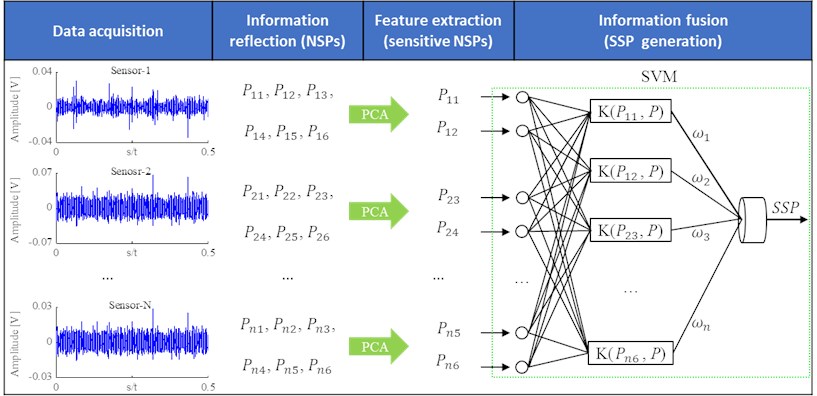
In the field of condition diagnosis, the excellent symptom parameters (SPs) must be defined to distinguish intelligently states of machinery as precisely as possible, and SPs must be able to reflect sensitively the characteristics of states [1, 8-11]. However, there is not an acceptable method for extracting SPs from signals measured in each state [12]. In order to increase the identification sensitivity, a SSP is defined with the function of the optimal classification hyper-plane which is obtained using SVM and all sensitive NSPs from multiple sensors, as shown in Figure 1. First, six NSPs are defined to extract the features of vibration information from each sensor. Second, PCA is used to evaluate and select sensitive NSPs of each sensor. Finally, a SVM is employed to fuse all sensitive NSPs from multiple sensors into an effective SSP.
Fig. 1Flow chart of the proposed method
2.1. Non-dimensional symptom parameters for reflecting vibration information
Many SPs have been defined in the pattern recognition field [13, 14]. In this study, six NSPs in the time domain are defined to reflect vibration information:
where (1, 2,…, ) is digital data of vibration signal, is the number of data. and are the mean value and the standard deviation:
where, ( 1, 2,…, ) is the valley data of vibration signal, is the number of data. and are the mean value and the standard deviation:
where, ( 1, 2,…, ) is the valley data of vibration signal, is the number of data. and are the mean value and the standard deviation.
2.2. Principal component analysis for selecting sensitive NSPs
Principal component analysis (PCA) is a multivariate statistical-analysis technique, in which a group of correlated variables are transformed into a new group of variables which are uncorrelated or orthogonal to each other [15, 16]. PCA can be done by eigenvalue decomposition of a data covariance matrix or the singular value decomposition of a data matrix. These decompositions are usually performed after mean centering the data for each attribute. The results of a PCA are usually discussed in terms of component scores and loadings [17]. In the last few years, PCA has been applied to process fault diagnosis [18-20].
The principle of using the PCA for selecting sensitive SPs is illustrated on the basis of a training data set of n samples (observations) and m variables (SPs). While these data are standardized by subtracting from its mean and dividing by its standard deviation, and the standardized data is denoted by a sample matrix , it is easy to obtain the covariance matrix with the eigenvector and the eigenvalue . Then a new component and its cumulative contribution rate are given as follows:
where, is each row vector of , and 1, 2,…,.
In general, when 85 %, , ,…, are called as principal components which contain most of the information and the discriminatory features. Moreover, the principal components load can express the correlation degree between principal component and original variable . Therefore, the comprehensive load of can be calculated as shown in Eq. (9). It has been proved that the larger the comprehensive load , the higher the sensitivity of the corresponding will be:
In this study, the comprehensive load of principal components is used as the evaluation standard of SP’s sensitivity, to select two sensitive NSPs which contain most of the vibration information each sensor.
2.3. Information fusion from multiple sensors using SVM
SVM is a classifier which uses statistical learning theory to create an optimal classification hyper-plane between the two classes and ensure that the distance between the boundary and the nearest data point in each class is maximized [21]. SVM can efficiently perform not only a linear classification but a non-linear classification using kernel function. In general, a classification hyper-plane can be expressed as follows:
where, is the sample vector, is the dimensional number of , is a vector represented the weight coefficients of , is a classification threshold.
Recently, almost all of practical applications of SVMs have employed different kernel functions, such as polynomial kernel and radial basis function (RBF) kernel, to achieve linear classifications in high-dimensional feature spaces. However, it is difficult to choose an appropriate kernel function and determine the parameters for a given value of the regularization and kernel parameters. In order to increase the enchantment of SVM, SVM is modified to permit minimum error and relax the condition for the optimal classification hyper-plane, and then soft margin SVM is proposed for a fuzzy inference system [11, 22].
In this study, the classification function of soft margin SVM is employed to achieve the optimization of fusing all sensitive NSPs selected from multiple sensors, and generate an effective SSP as the object of follow-on process. Then a SSP is defined as follows:
where, , ,…, are the sensitive NSPs selected from multiple sensors by PCA, and are the parameters of the optimal hyper-plane by training data.
3. Fuzzy diagnosis system
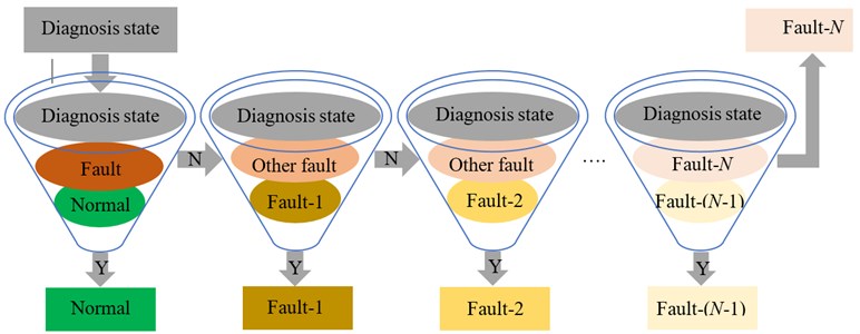
In Section 2, the proposed SSP, as the object of follow-on process, can improve excellently the identification sensitivity of two states. Moreover, it is very difficult to generate one SSP that is employed to identify simultaneously all states. However, in the cases of the practical diagnosis, there are many different fault states for the same mechanical equipment. Then possibility theory is introduced to build a sequential diagnosis system for fault detection and fault-type recognition, as shown in Fig. 2. Therefore, this section presents specifically two contents. Firstly, the principle of fuzzy inference is defined on the basis of possibility theory. Secondly, a diagnosis system is established to perform sequentially condition identification of many different faults.
3.1. Possibility theory for fuzzy inference
Possibility theory is a mathematical theory for making a fuzzy inference in processing ambiguous information [23, 24]. Recently, possibility theory has been applied to condition diagnosis in rotating machinery under varying rotating speeds to process the uncertain relationship between the symptoms and fault types [11, 25-27]. In the paper, for improving the recognition ability of ambiguous state, possibility theory is introduced to make a fuzzy inference for fault detection or fault-type recognition.
Fig. 2Fuzzy diagnosis system based on possibility theory
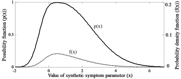
For fuzzy inference, the membership function of a SP is necessary [11, 25-27]. However, there are many methods for building the membership function of a SP. In this paper, a SSP, information fusion from multiple sensors by the proposed method in Section 2, is selected as the features for fault detection or fault-type recognition, and the possibility function of a SSP is regarded as the membership function to make a fuzzy inference. Since it is verified that each SSP follows the Weibull distribution, the possibility function of a SSP () can be obtained from probability density functions of the SSP () by the following formulae. Moreover, it is verified easily that the maximum value of the possibility function is 1:
and can be calculated as follows:
where, is the division number of the effective domain of a SSP , and are the mean and the standard deviation of the SSP, respectively. , and are the parameters of the shape, scale and location of Weibull distribution. Fig. 3 displays an illustration of the possibility function and the probability density function of a SSP.
Then it is easy to obtain the possibility functions of known states and diagnosis state. These known states, such as normal state and various kinds of fault states that have been diagnosed definitely, will be employed to regard the diagnosis standards as model states. Certainly, there are some faults that never occurred, and then these states are called “unknown state”. Therefore, there is no way to calculate directly the possibility function of unknown state. In order to extend the diagnostic capacity and enhance the identification sensitivity, an indirect method is proposed to obtain the possibility function of unknown state, as follows:
where, is the possibility functions of th known state, respectively, and is the number of all known states.
Fig. 3Possibility function and probability density function of a SSP
It is obvious that expresses the possibility function of unknown state except all known states. Then is regarded as the diagnosis standard of unknown state in the field of fuzzy inference.
Of course, it is required to define the matching approach of possibility functions between the model states and the diagnosis state for fuzzy inference. However, there are many matching methods defined in the field of fault diagnosis. In [11], the common area of the possibility functions between model state and diagnosis state was proposed as a useful matching method. However, the method must ensure a suitable range of symptom variable. Otherwise, the inference conclusion can be contorted. In [27], the possibility function value of a model state at the mean value of a diagnosis state was introduced to evaluate the degree of which the diagnosis state was the model state. The method that take the experience gained at one unit and popularize it in a whole area can ignore the non-symmetry distribution of symptom variable. Therefore, the paper proposes a novelty matching method based on Euclid close degree. Euclid close degree is one of the methods which express the proximity index of fuzzy sets [28], and can be calculated as follows:
where, and are the possibility functions of th model state and diagnosis state, and are the mean and the standard deviation of symptom variable of diagnosis state, respectively.
Moreover, these close degrees are normalized by:
Then the principle of selecting nearest is used to recognize the condition of diagnosis signal. The principle can use “if-then” rule as follows to explain the architecture of fuzzy inference.
Rule 1: if ,
then .
where is the close degree between model state and diagnosis state. is the possibility functions of the given model state. and express the conditions of diagnosis signal and model signal .
3.2. Sequential diagnosis approach
Fig. 2 describes the process of the sequential diagnosis system which is proposed in the paper. If there are types of faults that have occurred frequently, along with normal state, the diagnosis system needs to operate steps.
The first step of the diagnosis system is to detect whether mechanical condition is normal. Then the previous state that has been verified as “normal” is employed to confirm the possibility function of normal-model state. In the same way, N types of faults that have occurred frequently and been known definitely are united to establish the possibility function of fault-model state. Moreover, the possibility function of unknown-model state is obtained by the Eq. (15). When the information of the diagnosis state is put into the system, the close degrees between three model states and diagnosis state are calculated by the Eq. (17), and the fuzzy inference is performed by Rule 1. If the diagnosis state is judged as “normal state”, the diagnosis system automatically stops, and the diagnosis data is saved to optimize the possibility function of the future normal-model state. If the unknown state is shown, the system also stops, and we are reminded to investigate the real type of the diagnosis state. Otherwise, there is fault, and the system will come into the next step for fault-type identification. In the same way, each step only focuses to judge whether the diagnosis state is a type of fault from the second step until all fault-model states are performed sequentially.
4. Experimental verification
To verify the feasibility and effectiveness of the proposed fuzzy diagnosis method for detecting and distinguishing multi-fault state, the fault diagnosis of roller bearing is studied by using the real data obtained from test bench.
4.1. Experimental system
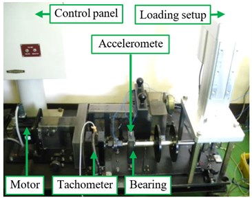
Fig. 4 shows the experimental system which is driven by a variable speed 3AC motor with speeds up to 2000 rpm. In order to research fault diagnosis of roller bearing in a real plant, it is equipped with loading setup (Model: RCS2-RA13R) which can transport the power of a fixed or varied load up to 2 T. The bearings (Type: UK204) are utilized, and the specification of the bearings is listed in Table 1.
Fig. 4The rotating machine for fault diagnosis
In the case of the practical diagnosis, three single-fault states, namely, the outer race defect (O), the inner race defect (I), the rolling element defect (R), and two multi-fault states, such as the outer race-rolling element defect (OR), and the inner race-rolling element defect (IR), have occurred frequently in a roller bearing. In order to research whether these faults of roller bearing are detectable at an early stage, especially multi-fault states, the faults were artificially made with the use of a wire-cutting machine, and the defect sizes were the same: the width was 0.3 mm and the depth was 0.15 mm. Pictures of five fault states are shown in Fig. 5.
Fig. 5Defect types for roller bearing fault diagnosis test
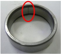
a) Outer race defect (O)
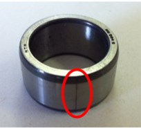
b) Inner race defect (I)
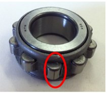
c) Roller element defect (R)
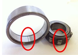
d) Outer race-rolling element defect (OR)
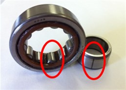
e) Inner race-rolling element defect (IR)
Table 1Specification of the bearing
Contents | Parameter | Contents | Parameter |
Outer diameter | 47 mm | Roller diameter | 7 mm |
Inner diameter | 20 mm | Number of rollers | 11 |
Width | 14 mm | Contact angle | 0 rad |
In this work, three accelerometers (Type: PCB MA352A60; Sensitivity: 10 mV/g; Frequency: 5-60000 Hz) were mounted on the three directions (horizontal, vertical and axial direction) of the bearing housing to acquire the vibration signals with a sampling frequency of 50 kHz, and the sampling time was 20 sec. As the rotating machine usually works at a constant speed and a fixed load, the vibration signals of normal state and five faults were measured at a rotation speed of 1000 rpm and 120 kg load.
4.2. Diagnosis system building
In order to fully analyze signal feature, these signals measured from different operating condition and different direction were firstly normalized using the following equation for diagnosis:
where and were the mean and standard deviation of an original signal .
Second, each signal was divided into 120 parts. Each part contained 8192 sampling points for high-pass filtering with 10 kHz cut-off frequency and calculation of six NSPs defined in Section 2.1. Then 120 samples of NSPs were split into two sets: 40 samples for training and the remaining 80 samples for testing.
Since six different operating conditions of roller bearing were performed in the experiment, the diagnosis system was designed to undergo five stages for fault detection and fault-type recognition, as shown in Fig. 6. Then in each stage, 40 samples of NSPs corresponding to two states were used to select two sensitive NSPs from each sensor by PCA as shown in Section 2.2. As an example, parts of the selection results from six NSPs in horizontal direction are shown in Table 2. Similarly, higher sensitive NSPs were also selected in vertical and axial directions, as shown in Table 3.
Fig. 6Flowchart of sequential diagnosis based on the test experiment
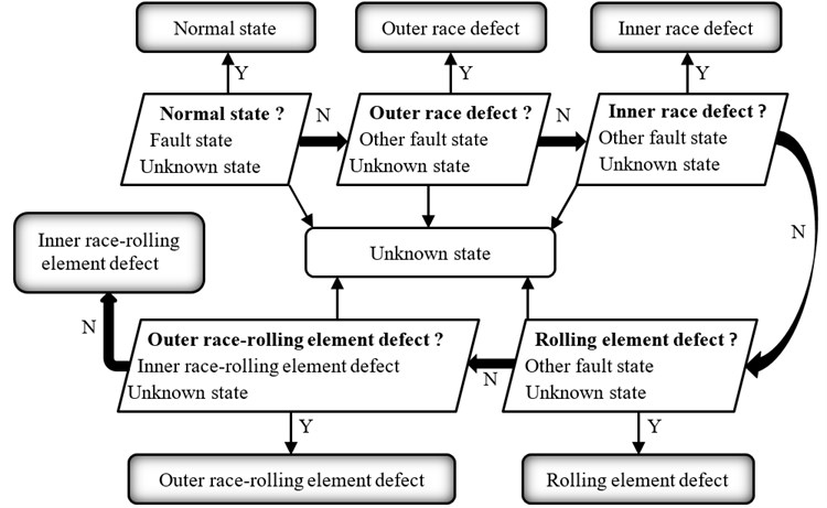
Table 2Higher sensitive NSPs selected by PCA in horizontal direction
Each stage | Two states identified in each stage | Comprehensive load C of NSPs in PCA | Higher sensitive NSPs | ||||||
One state | Other state | ||||||||
1 | Normal state | Fault state | –0.09 | –0.6 | 0.76 | 0.13 | 0.97 | –0.7 | , |
2 | Outer race defect | Other fault state | –0.71 | –0.11 | 0.5 | 0.79 | –0.4 | 0.81 | , |
3 | Inner race defect | Other fault state | –0.16 | 0.89 | 0.77 | 0.25 | –0.70 | –0.18 | , |
4 | Rolling element defect | Other fault state | –0.02 | –0.27 | 0.84 | 0.16 | 0.90 | –0.8 | , |
5 | Outer race-rolling element defect | Inner race-rolling element defect | –0.43 | –0.39 | 0.39 | 0.60 | –0.38 | 0.72 | , |
In each stage, higher sensitive NSPs selected from three directions were used as input layer of soft margin SVM, and two states that would be identified were set to become output layer and associate with labels: 1 for the goal state and –1 for the other state. When soft margin SVM was trained, the parameters and of the optimal hyper-plane were confirmed, and the definition of the effective SSP in the stage was achieved. Table 4 is the definitions of effective SSPs in each stage.
Then the possibility functions of the model states in each stage were obtained by the Eq. (12) and Eq. (15). Thus, the diagnosis system was built to perform sequentially fault detection and fault-type recognition.
Table 3Higher sensitive NSPs from three directions by PCA
Each stage | Two states identified in each stage | Higher sensitive NSPs from each direction | |||
One state | Other state | Horizontal | Vertical | Axial | |
1 | Normal state | Fault state | , | , | , |
2 | Outer race defect | Other fault state | , | , | , |
3 | Inner race defect | Other fault state | , | , | , |
4 | Rolling element defect | Other fault state | , | , | , |
5 | Outer race-rolling element defect | Inner race-rolling element defect | , | , | , |
Note: (1, 2,…, 6) are used to express six NSPs from vertical and axial directions | |||||
Table 4Synthetic symptom parameters (SSPs) in each stage
Each stage | Synthetic symptom parameter |
1 | |
2 | |
3 | |
4 | |
5 |
4.3. Experimental verification
To verify the diagnostic capability of the method proposed in this study, the remaining 80 samples of NSPs from each operating condition and each direction were also split equally into four sets. Four test data sets were labeled by test-1, test-2, test-3, test-4. As an example, when the data of Test-1 were performed in the same procedure, and input into the diagnosis system, the close degrees between three model states of diagnosis system and test state were calculated in each stage, and the results of fuzzy inferences were output, as shown in Table 5.
Table 5Close degrees in each stage and diagnosis results of Test-1
Each stage | Model state in diagnosis system | Close degree between model state and test state | |||||
Test state | |||||||
N | O | I | R | OR | IR | ||
1 | Normal state (N) | 0.891 | 0.154 | 0.178 | 0.209 | 0.192 | 0.234 |
Fault state | 0.103 | 0.827 | 0.795 | 0.732 | 0.800 | 0.729 | |
Unknown state | 0.006 | 0.019 | 0.027 | 0.059 | 0.008 | 0.047 | |
2 | Outer race defect (O) | 0.796 | 0.160 | 0.137 | 0.274 | 0.138 | |
Other fault state | 0.201 | 0.825 | 0.848 | 0.709 | 0.826 | ||
Unknown state | 0.003 | 0.015 | 0.015 | 0.017 | 0.046 | ||
3 | Inner race defect (I) | 0.816 | 0.211 | 0.116 | 0.281 | ||
Other fault state | 0.144 | 0.758 | 0.852 | 0.706 | |||
Unknown state | 0.040 | 0.031 | 0.032 | 0.013 | |||
4 | Rolling element defect (R) | 0.839 | 0.208 | 0.255 | |||
Other fault state | 0.147 | 0.751 | 0.720 | ||||
Unknown state | 0.024 | 0.041 | 0.025 | ||||
5 | Outer race-rolling element defect (OR) | 0.808 | 0.196 | ||||
Inner race-rolling element defect (IR) | 0.172 | 0.781 | |||||
Unknown state | 0.020 | 0.023 | |||||
Judge state by close degrees | N | O | I | R | OR | IR | |
Similarly, the data of Test-2, Test-3, Test-4 were independently used to input into the diagnosis system, and the diagnosis results are displayed in Table 6.
Table 6Diagnosis results by the proposed method
Test set | Diagnosis project | Test state from each test set | |||||
N | O | I | R | OR | IR | ||
Test-1 | Diagnostic progress | 1 | 2 | 3 | 4 | 5 | 5 |
Close degree | 0.891 | 0.796 | 0.816 | 0.839 | 0.808 | 0.781 | |
Judge state | N | O | I | R | OR | IR | |
Test-2 | Diagnostic progress | 1 | 2 | 3 | 4 | 5 | 5 |
Close degree | 0.853 | 0.809 | 0.769 | 0.803 | 0.770 | 0.815 | |
Judge state | N | O | I | R | OR | IR | |
Test-3 | Diagnostic progress | 1 | 2 | 3 | 4 | 5 | 5 |
Close degree | 0.867 | 0.782 | 0.784 | 0.815 | 0.793 | 0.799 | |
Judge state | N | O | I | R | OR | IR | |
Test-4 | Diagnostic progress | 1 | 2 | 3 | 4 | 5 | 5 |
Close degree | 0.870 | 0.773 | 0.787 | 0.798 | 0.766 | 0.805 | |
Judge state | N | O | I | R | OR | IR | |
Diagnosis accuracy | 100 % | 100 % | 100 % | 100 % | 100 % | 100 % | |
100 % | |||||||
4.4. Experimental comparison
To verify the effectiveness of synthetic symptom parameter (SSP) on the basis of vibration information fusion from multiple sensors, vibration information of single sensor was planned to fuse an object of follow-on process. Then higher sensitive NSPs from single direction as shown in Table 3 were respectively used to perform in the same procedure. The diagnosis results on the basis of vibration information from horizontal, vertical or axial direction are shown in Table 7, Table 8, Table 9, respectively.
Table 7Diagnosis results based of vibration information from horizontal direction
Test set | Diagnosis project | Test state from each test set | |||||
N | O | I | R | OR | IR | ||
Test-1 | Diagnostic progress | 1 | 2 | 5 | 4 | 2 | 5 |
Close degree | 0.747 | 0.619 | 0.735 | 0.621 | 0.688 | 0.700 | |
Judge state | N | O | IR | R | O | IR | |
Test-2 | Diagnostic progress | 1 | 2 | 3 | 5 | 2 | 3 |
Close degree | 0.789 | 0.722 | 0.698 | 0.743 | 0.713 | 0.662 | |
Judge state | N | O | I | IR | O | I | |
Test-3 | Diagnostic progress | 1 | 5 | 3 | 4 | 5 | 3 |
Close degree | 0.804 | 0.684 | 0.750 | 0.617 | 0.756 | 0.627 | |
Judge state | N | OR | I | R | OR | I | |
Test-4 | Diagnostic progress | 1 | 2 | 5 | 4 | 2 | 5 |
Close degree | 0.773 | 0.718 | 0.742 | 0.793 | 0.682 | 0.736 | |
Judge state | N | O | IR | R | O | IR | |
Diagnosis accuracy | 100 % | 75 % | 50 % | 75 % | 25 % | 50 % | |
62.5 % | |||||||
The diagnosis results from Table 6 have shown that all test states have been diagnosed correctly, and close degrees between model states and test states have remained above 0.75. However, the results from Table 7, Table 8 and Table 9 have shown that all fault states have been detected correctly, but more erroneous judges have happened for fault-type recognition, especially multi-fault states. It is very obvious that the diagnostic capability and effectiveness based on information fusion from multiple direction s are better than single direction.
Table 8Diagnosis results based of vibration information from vertical direction
Test set | Diagnosis project | Test state from each test set | |||||
N | O | I | R | OR | IR | ||
Test-1 | Diagnostic progress | 1 | 2 | 3 | 5 | 2 | 5 |
Close degree | 0.785 | 0.627 | 0.671 | 0.609 | 0.637 | 0.654 | |
Judge state | N | O | I | IR | O | IR | |
Test-2 | Diagnostic progress | 1 | 2 | 5 | 5 | 5 | 5 |
Close degree | 0.811 | 0.786 | 0.736 | 0.696 | 0.683 | 0.712 | |
Judge state | N | O | IR | IR | OR | IR | |
Test-3 | Diagnostic progress | 1 | 2 | 3 | 4 | 2 | 4 |
Close degree | 0.803 | 0.784 | 0.659 | 0.664 | 0.650 | 0.648 | |
Judge state | N | O | I | R | O | R | |
Test-4 | Diagnostic progress | 1 | 2 | 5 | 4 | 5 | 3 |
Close degree | 0.798 | 0.741 | 0.653 | 0.710 | 0.644 | 0.737 | |
Judge state | N | O | IR | R | OR | I | |
Diagnosis accuracy | 100 % | 100 % | 50 % | 50 % | 50 % | 50 % | |
67.7 % | |||||||
Table 9Diagnosis results based of vibration information from axial direction
Test set | Diagnosis project | Test state from each test set | |||||
N | O | I | R | OR | IR | ||
Test-1 | Diagnostic progress | 1 | 2 | 3 | 4 | 2 | 3 |
Close degree | 0.715 | 0.699 | 0.628 | 0.730 | 0.710 | 0.756 | |
Judge state | N | O | I | R | O | I | |
Test-2 | Diagnostic progress | 1 | 5 | 3 | 5 | 2 | 4 |
Close degree | 0.747 | 0.714 | 0.650 | 0.708 | 0.663 | 0.598 | |
Judge state | N | OR | I | IR | O | R | |
Test-3 | Diagnostic progress | 1 | 5 | 5 | 4 | 5 | 4 |
Close degree | 0.679 | 0.635 | 0.678 | 0.671 | 0.705 | 0.629 | |
Judge state | N | O | IR | R | OR | R | |
Test-4 | Diagnostic progress | 1 | 2 | 5 | 5 | 2 | 5 |
Close degree | 0.653 | 0.690 | 0.702 | 0.733 | 0.661 | 0.735 | |
Judge state | N | O | IR | IR | O | IR | |
Diagnosis accuracy | 100 % | 50 % | 50 % | 50 % | 25 % | 25 % | |
50 % | |||||||
5. Conclusions
To improve the ambiguous relationship between multi-fault state and the vibration feature, especially at an early stage, and increase the accuracy of fault detection and fault-type recognition, a fuzzy diagnosis method for multi-fault state was presented on the basis of information fusion from multiple sensors, and the effectiveness was demonstrated experimentally. The main conclusions were obtained as follows.
1) Multiple sensors demonstrate a predictable response to complementary information when the sensors are mounted on different locations for diagnosing the same equipment or parts. Vibration information from multiple sensors can process the effective features of multi-fault state, even if at an early stage.
2) It is proven to be effective and improve the robustness of diagnosis system that soft margin SVM is used to fuse vibration information from multiple sensors.
3) The efficiency of fuzzy diagnosis proposed in the paper has been verified by applying it to a practical diagnosis for detecting and distinguishing multi-fault states of bearing. The perfect performance is attributed primarily to effective features from multiple sensors, soft margin SVM’s generalization capability, SSP’s high sensitivity, and possibility theory for fuzzy inference.
For future works, the method proposed in this paper will be expanded to perform in the vehicle field, the focus is how to extract fault feature under the influence of noise and complex driving conditions, and build the threshold model of fuzzy diagnosis.
References
-
Chen P. Foundation and Application of Condition Diagnosis Technology for Rotating Machinery. Sankeisha Press, Japan, 2009.
-
Hu H., Gehin A., Bayart M. An extended qualitative multi-faults diagnosis from first principles. I: theory and modelling. Joint 48th IEEE Conference on Decision and Control and 28th Chinese Control Conference, 2009, p. 1008-1013.
-
Bachschmid N., Pennacchi P., Vania A. Identification of multiple faults in rotor systems. Journal of Sound Vibration, Vol. 254, 2002, p. 327-366.
-
Li Z., Yan X., Yuan C., Peng Z., et al. Virtual prototype and experimental research on gear multi-fault diagnosis using wavelet-autoregressive and principal component analysis method. Mechanical Systems and Signal Processing, Vol. 25, 2011, p. 2589-2607.
-
Lal M., Tiwari R. Multi-fault identification in simple rotor-bearing-coupling systems based on forced response measurements. Mechanism and Machine Theory, Vol. 51, 2012, p. 87-109.
-
Liu Z., Cao H., Chen X., He Z., Shen Z. Multi-fault classification based on wavelet SVM with POS algorithm to analyze vibration signals from rolling element bearings. Neurocomputing, Vol. 99, 2013, p. 399-410.
-
Jiang H., Li C., Li H. An improve EEMD with multi-wavelet packet for rotating machinery multi-fault diagnosis. Mechanical Systems and Signal Processing, Vol. 36, 2013, p. 225-239.
-
Matuyama H. Diagnosis algorithm. Journal of JSPE, Vol. 75, 1991, p. 35-37.
-
Chen P., Toyota T. Fuzzy diagnosis and fuzzy navigation for plant inspection and diagnosis robot. Proceedings of FUZZ-IEEE/IFES, Vol. 1, 1995, p. 185-193.
-
Fukunaga K. Introduction to Statistical Pattern Recognition. Academic Press, San Diego, CA, USA, 1972.
-
Xue H., Li Z., Li K., Wang H., Chen P. Intelligent diagnosis method for centrifugal pump system using vibration signal and support vector machine. Shock and Vibration, 2014, p. 407570.
-
Richardson J. J. Artificial Intelligence in Maintenance. Noyes Publications, New Jersey, USA, 1985.
-
Wang H., Chen P. Fuzzy diagnosis method for rotating machinery in variable rotating speed. IEEE Sensors Journal, Vol. 11, Issue 1, 2011, p. 23-34.
-
Zhu J., Li Z., Li K., Xue H., Chen P. Intelligent method of condition diagnosis for rotating machinery using relative ratio symptom parameter and Bayesian network. Advanced Science Letters, Vol. 4, 2011, p. 2532-2537.
-
Edward Jackson J. A User’s Guide to Principal Components. John Wiley and Sons Inc., 1991.
-
Jolliffe I. T. Principal Component Analysis. Springer-Verlag, New York Inc., 1986.
-
Abdi H., Williams L. J. Principal component analysis. Wiley Interdisciplinary Reviews: Computational Statistics, Vol. 2, Issue 10, 2010, p. 433-459.
-
Johannesmeyer M. C., Singhal A., Seborg D. E. Pattern matching in historical data. AIChE Journal, Vol. 48, 2002, p. 2022–2038.
-
Kano M., Tanaka S., Hasebe S., Hashimoto I., Ohno H. Monitoring independent components for fault detection. AIChE Journal, Vol. 49, 2003, p. 969-976.
-
Lu N., Wang F., Gao F. Combination method of principal component and wavelet analysis for multivariate process monitoring and fault diagnosis. Industrial and Engineering Chemistry Research, Vol. 42, 2003, p. 4198-4207.
-
Gunn S. R. Support Vector Machines for Classification and Regression. Technical Report, University of Southampton, 1998.
-
Xue H., Wang H., Chen P., Li K., Song L. Automatic diagnosis method for structural fault of rotating machinery based on distinctive frequency components and support vector machine under varied operating conditions. Neurocomputing, Vol. 116, Issue 20, 2012, p. 326-335.
-
Zadeh L. A. Fuzzy sets. Information and Control, Vol. 8, Issue 3, 1965, p. 338-353.
-
Dubois D., Prade H. Possibility Theory: An Approach to Computerized Processing of Uncertainty. Plenum Press, New York, USA, 1988.
-
Chen P., Toyota T. Method of failure detection by possibility theory and Dempster and Shafer probability theory. Journal of Kitakyushu Medical and Engineering Cooperative Association, Vol. 9, 1998, p. 1-4.
-
Chen P., Toyota T. Sequential fuzzy diagnosis for plant machinery. JSME International Journal Series C Mechanical Systems, Machine Elements and Manufacturing, Vol. 46, Issue 3, 2003, p. 1121-1129.
-
Wang H., Chen P. Intelligent diagnosis method for rolling element bearing faults using possibility theory and neural network. Computers and Industrial Engineering, Vol. 60, 2011, p. 511-518.
-
Xie J., Liu C. Fuzzy Mathematics Method and its Application. Huazhong University of Science and Technology Press, 2005.
Cited by
About this article

This project is supported by the National Natural Science Foundation of China (Grant No. 51575241, 51305111), Six Talent Peaks Project in Jiangsu Province (Grant No. 2012-ZBZZ-030), the Foundation of Jiangsu University (Grant No. 14JDG123), and the Key Laboratory of Road Vehicle New Technology Application in Jiangsu Province (Grant No. BM20082061508).
The first author contributed to design and implement the methodology and wrote the manuscript. The other authors carried out the experiments and analyzed the results.
