Abstract
Sealed deep groove ball bearings (SDGBBs) are employed to perform the relevant duties of in-wheel motor. However, the unique construction and complex operating environment of in-wheel motor may aggravate the occurrence of SDGBB faults. Therefore, this study presents a new intelligent diagnosis method for detecting SDGBB faults of in-wheel motor. The method is constructed on the basis of optimal composition of symptom parameters (SPOC) and support vector machines (SVMs). SPOC, as the objects of a follow-on process, is proposed to obtain from symptom parameters (SPs) of multi-direction. Moreover, the optimal hyper-plane of two states is automatically obtained using soft margin SVM and SPOC, and then using multi-SVMs, the system of intelligent diagnosis is built to detect many faults and identify fault types. The experiment results confirmed that the proposed method can excellently perform fault detection and fault-type identification for the SDGBB of in-wheel motor in variable operating conditions.
1. Introduction
In-wheel motor is employed to drive electric vehicle, especially electric bicycles. It usually converts produced electricity into other forms of energy to provide power to vehicle wheel. However, the unique construction and complex operating environment of in-wheel motor may aggravate the occurrence of bearing faults. The bearing faults may cause the performance breakdown of in-wheel motor, and affect the driving safety of a vehicle, and further, serious consequences may be injurious to personal safety. Therefore, it is very important to monitor and diagnose the bearing faults of in-wheel motor [1].
Currently, many literatures are concerned with fault diagnosis of motor [1-7]. An intelligent diagnosis based on an adaptive neuro-fuzzy inference system was presented to identify electrical faults of in-wheel motor [1]. The parameter estimation method of a multipole permanent magnet synchronous motor (PMSM) was presented to solve interturn short circuit fault [2]. A novel permanent magnetic angular acceleration sensor was developed to measure the instantaneous angular acceleration for status monitoring and fault diagnosis of a single-phase asynchronous motor [3]. A symbolic dynamic method is presented for health monitoring of permanent magnet synchronous motors (PMSMs), which involves abstraction of a qualitative description from a dynamical system representation of the PMSM [4]. A novel approach based on tracking characteristic orders of stator current using Vold-Kalman filter is proposed to detect the partial demagnetization fault in PMSMs running at nonstationary conditions. The amplitude of envelope of the fault characteristic orders is used as fault indictor [5]. The above methods mainly researched the diagnosis methods of electrical faults of a motor. However, there is little focus on bearing faults of a motor, especially in-wheel motor.
Certainly, there are many literatures concerned with fault diagnosis of rolling bearing. Statistical symptom parameters and the fuzzy neural network were used to judge automatically the bearing faults [8, 9]. Statistical analysis was used to detect bearing faults [10, 11]. Several autoregressive modeling techniques were compared to perform the effectiveness of fault diagnosis for rolling element bearings [12]. Fourier transform (FT), wavelet transform (WT), empirical mode decomposition (EMD), short time Fourier transform (STFT) and compressed sensing (CS) theory are used to extract the fault features of rolling bearing [13-16].
Moreover, in the field of condition monitoring and machinery diagnosis, symptom parameter (SP) is extremely important and effective tool. If we can find good symptom parameters which sensitively reflect the feature of the machine states, automatic diagnosis for mechanical failure is possible [17-20]. However, in many cases of the condition diagnosis for rotating machinery in a real plant, there are many problems as follows: (1) Effective SPs cannot be easily found because of too many fault categories [19, 21, 22]; (2) The sensitivity of SP is not high under the influence of noise and operating conditions to be diagnosed machine [23, 24]; (3) Traditional condition diagnosis methods such as neural networks, bee colony algorithm, other algorithms based on statistical learning require a large number of training samples [25-32]. However, in most cases of practical machinery, measured signals are not so sufficient for the condition of learning data. The intelligent methods, namely neural networks, genetic algorithms, etc., often cannot converge when learning, so the work of condition diagnosis is in passive situation.
To resolve the above problems, this paper proposes a condition diagnosis method based on soft margin SVMs and SPOC. SPs can be calculated by using the measured vibration signals from three directions, and principal component analysis (PCA) is used to select sensitive SPs of each direction, and to build optimal composition of symptom parameters (SPOC). Finally, intelligent diagnosis method using SPOC and soft margin SVMs is proposed to diagnose bearing faults of in-wheel motor.
2. Feature extraction of bearing fault
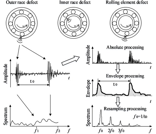
In general, sealed deep groove ball bearings (SDGBBs) are employed to perform the relevant duties of in-wheel motor. Since the design structure and operating environment of in-wheel motor are different than common motor, the bearing locals of in-wheel motor may aggravate the abrasion process. By analyzing some real cases of in-wheel motor, localized defects of SDGBB usually occur in the outer race, the inner race, and the roller as common bearing. However, the difference is that outer race and inner race of SDGBB are curved surface, but ones of common bearing are flat surface. Here, to understand easily the proposed method, the elements of localized defects are still used to define the fault types of SDGBB. Then typical faults of SDGBBs are so-called “outer race defect (ORD)”, “inner race defect (IRD)”, “rolling element defect (RED)”.
2.1. Feature extraction of bearing faults
It is generally known that the localized defects of each bearing-element generate a series of shock vibrations every time a running roller passes over the surfaces of the defects, and these vibrations occur at bearing characteristic frequencies, which are estimated based on the geometry of the bearing, its rotational speed, and the location of the defect. Moreover, the bearing characteristic frequencies capture in high-frequency domain [19]. By identifying the type of the occurring bearing characteristic frequency, envelope processing is used to extract the feature spectrum of bearing faults. Certainly, upper-envelope, lower envelope and full envelope are applied to detect faults. In this paper, absolute envelope processing is proposed, as shown in Fig. 1.
Here, ORD is used as example to introduce the absolute envelope processing. Firstly, band-pass filter is used to remove the noise signal outside the frequency domain captured by bearing faults. Where, expresses the pass-time of the defect, and are the cut-off frequencies of original spectrum. Secondly, the filtered signal is processed through absolute envelope, then to obtain an envelope signal which obviously presents shock characteristics. Finally, lower frequency is used to resample from envelope signal to a new wave, then the new wave is transformed into the frequency domain by fast Fourier transform (FFT). The pass-frequency corresponding to the pass-time of the defect and its harmonic pass-frequencies 2, 3, … will capture in the spectrum of the new wave. When a pure rolling motion is assumed, ball pass frequency outer (BPFO), ball pass frequency inner (BPFI) and ball spin frequency (BSF) can be estimated on the basis of the geometry of the bearing, its rotational speed, and the location of the defect [33-35].
Fig. 1Feature spectrums extraction using envelope processing
Ball pass frequency outer (BPFO) can be calculated as follows:
Ball pass frequency inner (BPFI) can be calculated as follows:
Ball spin frequency (BSF) can be calculated as follows:
where is the number of rolling elements, is the rotating frequency (Hz), is the diameter of rolling elements (mm), is the pitch diameter (mm), and is the contact angle of the rolling element (rad).
In practice, some sliding motion may occur on the working process of rolling bearing. Then slight deviation of the characteristic frequency locations can be caused. Therefore, these pass-frequencies calculated by above-mentioned equations should be regarded as theoretical value only, and the frequency region adjacent to theoretical value will be focused to identify the fault-type of rolling bearing.
2.2. Symptom parameters of fault feature
To perform intelligent diagnosis in the operating process, it is necessary that symptom parameters (SPs) are used to represent the fault features of machinery or parts. In the field of condition diagnosis, many SPs have been defined for fault diagnosis and fault-type identification [17, 19, 36]. Since bearing fault is a typical impact fault, and its characteristic frequencies generally capture in high-frequency domain, six dimensionless SPs in frequency domain are selected to represent the bearing fault features of in-wheel motor in this research, the signals processed by the absolute envelope method are used to calculate these SPs, as follows:
where, is the number of spectrum line, is the frequency, is the power spectrum. and .
2.3. Principal component analysis for Selecting sensitive SPs
Principal component analysis (PCA) is a multivariate statistical-analysis technique, in which a group of correlated variables are transformed into a new group of variables which are uncorrelated or orthogonal to each other [37, 38]. PCA can be done by eigenvalue decomposition of a data covariance matrix or the singular value decomposition of a data matrix. These decompositions are usually performed after mean centering the data for each attribute. The results of a PCA are usually discussed in terms of component scores and loadings. Recently, PCA has been applied to process fault diagnosis [39, 40].
To improve the rapidity of identifying targets, the PCA principle is illustrated for selecting two sensitive SPs from six SPs selected primitively on the basis of a training data set of samples (observations) and variables (SPs). While these data are standardized by subtracting from its mean and dividing its standard deviation, and the standardized data is denoted by a matrix , it is easy to obtain the covariance matrix with the eigenvector and the eigenvalue . Then a new component and its cumulative contribution rate are given as follows:
where is each row vector of and .
In general, when the values of are more than 85 %, the corresponding components are called as principal components which contain most of the information and the discriminatory features. Here, the value corresponding to the minimum value of is labeled with . Moreover, the principal components load can express the correlation degree between principal component and original variable . Therefore, the comprehensive load of can be calculated as follows:
It has been proved that the larger the comprehensive load , the higher the sensitivity of the corresponding will be. In this study, the comprehensive load of principal components is used to select the sensitive SPs as the evaluation standard of SP’s sensitivity, and then select two sensitive SPs are selected to contain most of the vibration information each direction. Finally, two sensitive SPs from each direction are combined to build optimal composition of symptom parameters (SPOC).
3. Sequential diagnosis method based on soft margin SVMs
3.1. Soft margin SVMs
SVM is a classifier which uses statistical learning theory to create an optimal classification hyper-plane between the two classes and ensure that the distance between the boundary and the nearest data point in each class is maximized [41-46]. SVM can efficiently perform not only a linear classification but a non-linear classification using kernel function. In general, a classification hyper-plane can be expressed as follows:
where, is the sample vector, is the dimensional number of , is a vector represented the weight coefficients of , is a classification threshold.
Recently, almost all of practical applications of SVMs have employed kernel functions to achieve linear classifications in high-dimensional feature spaces. However, it is difficult to choose an appropriate kernel function and determine the parameters for a given value of the regularization and kernel parameters. In order to increase the enchantment of SVM, SVM is modified to permit minimum error and relax the condition for the optimal classification hyper-plane, soft margin SVM is proposed for a fuzzy inference system [47, 48].
3.2. Sequential diagnosis system
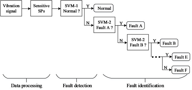
Sequential diagnosis system is presented to monitor machine condition and identify fault types, as shown in Fig. 2. The first soft margin SVM is used to detect faults while the others are used to identify sequentially fault types. Moreover, SPOCs are employed as the object of follow-on process to put a SVM in each step, then obtain the optimal hyper-plane until whole diagnosis system is established.
Fig. 2Sequential diagnosis system based on SPs and SVMs
4. Verification experiment
4.1. Experimental system
Fig. 3 shows the experimental equipment for the bearing fault test of in-wheel motor, and the place of accelerometer and diagnosis bearing of in-wheel motor. The parameters of the in-wheel motor is listed that rated power is 350 W, rated voltage is 48 V, rated speed is 300 rpm. 6202RS bearings were utilized, which information are listed in Table 1. In order to research whether the most commonly occurring bearing faults of in-wheel motor are detectable, the faults of diagnosis bearings were artificially made using a wire-cutting machine in the ORD, IRD or RED, and the defect sizes were the same: the width was 0.2 mm and the depth was 0.1 mm. Moreover, a 3-axis accelerometer (Type: CXL25GP3; Sensitivity: 80 mV/g; Range: ±25 g) was mounted on the holder which was fixed the stator axis of in-wheel motor. The vibration signals of normal state and three faults were measured with a sampling frequency of 204.8kHz, and the sampling time is 20 s. Moreover, when the operating speed was operated from 200 to 300 rpm, BPFO, BPFI and BSF are 6.1-9.1 Hz, 20.6-30.9 Hz, and 4.3-6.4 Hz, respectively.
Fig. 3Experimental equipment for fault diagnosis
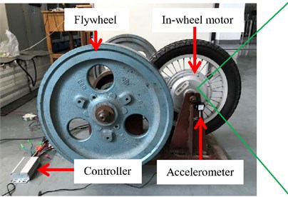
a) Experimental bench of in-wheel motor
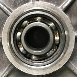
b) Sealed deep groove ball bearing
Table 1Necessary parameters of sealed deep groove ball bearing
Contents | Parameters | Contents | Parameters |
Specification | 6202RS | Width | 11 mm |
Outer diameter | 35 mm | Roller diameter | 5 mm |
Inner diameter | 15 mm | Roller’s number | 8 |
4.2. Data processing
The vibration signals collected from bearing experiment were divided into 60 data samples, respectively. Each data sample was actually a data series containing 65536 data points, and was processed by absolute envelope method. Here, band-pass filter (10 kHz was lower cut-off frequency and 100 kHz was upper cut-off frequency) was selected, and new data sample was measured by with a new resampling frequency of 2 kHz from the curve of absolute envelope. Finally, new data sample was used to calculate six SPs. Therefore, 60 data samples were obtained in each condition.
According to the test experiment and the sequential diagnosis method as shown in Fig. 2, the diagnostic system was designed four steps. The goal of the first step will focus whether the diagnosis condition is normal state (N). If the diagnosis condition is N, the system will stop. Otherwise, the system will come in the second step, and identify whether it is ORD. If not, diagnosis process will push forward the third step, and judge whether it is IRD. Similarly, RED will be distinguished in the fourth step. Certainly, there are more fault types in real plant, more steps can be continued in sequential diagnosis system. In order to fleetly detect fault and identify fault type, two SPs have been selected to aim toward the goal of each step by PCA from each direction, as shown in Table 2. Here, , and ( 1, 2,…, 6) are used to reflect the corresponding SPs from vertical, horizontal and axial directions, respectively. Then the SPOCs are confirmed in each step.
Table 2Selection results of sensitive SPs from each direction in each step
Each step | Diagnosis goal | Selection results from each direction | ||
Vertical direction | Horizontal direction | Axial direction | ||
1 | N | , | , | , |
2 | ORD | , | , | , |
3 | IRD | , | , | , |
4 | RED | , | , | , |
4.3. Diagnosis system establishment and diagnosis results
To verify the effectiveness of the proposed method for diagnosing the faults of motor bearing, 30 data samples obtained from three directions were used to obtain 30 datasets of SPOCs in each condition, then to train the diagnosis system. Firstly, the establishment of the diagnosis system was described. In the first step, N was the diagnosis goal as one class with label 1. Then each and its status label 1 (1, 2, …, 30) were built to identify whether it is . Another class was abnormal state (UN) which included three bearing faults of ORD, IRD and RED with label –1, each SPOC and its status label –1 ( 1, 2, …, 90) were built to affirm whether it is UN. Secondly, the SPOCs and its status labels of N and UN were combined to input into a SVM as the training data, shown as and . Since soft margin SVM was adopted, minimum error and relax coefficient were designed. In this research, it was proved to be optimal that minimum error was 5 % and relax coefficient was 0.05. Moreover, the weight coefficients of and classification threshold were determined, then the optimal classification hyper-plane between N and UN was obtained, as shown in Table 3. Similarly, the goal state of the second step was ORD to label with 1, other faults (UORD) were regarded as another class with label –1. In the third step, IRD was designed for the diagnosis goal with label 1, other faults (UIRD) were regarded as another class with label –1. In the fourth step, RED was designed for diagnosis goal with label 1, other faults (URED) were regarded as another class with label –1. Then the training data of each step were determined to obtain the corresponding optimal classification hyper-plane, respectively. The optimal classification hyper-plane of each step can be expressed as shown in Table 3. Then the diagnosis system was established.
Table 3Optimal classification hyper-plane of each step
Each step | Diagnosis goal | Optimal classification hyper-plane |
1 | N | |
2 | ORD | |
3 | IRD | |
4 | RED |
Secondly, other 30 data samples of each condition were used to test the performance of the diagnosis system, then SPOCs of each condition in each step were selected according to Table 2. Here, the test data of ORD was used to introduce the proposed method. In the first step, the test data with SPOC was input into the first SVM classifier, it was obtained that the probability which the diagnosing condition was N state was 12.5 %. Obviously, the diagnosing condition was judged to be state, and then the diagnosis system turned into the second step. Therefore, SPOC was used to identify whether it is ORD state. When inputting the new test data into the second SVM, the probability which the diagnosing condition was ORD state was 90.9 %, and the diagnosis system stopped. It is correct that the diagnosing condition was judged to be ORD state. Similarly, the test data of other diagnosing conditions were input to the diagnosis system respectively, the diagnosis results were shown in Table 4.
Table 4Diagnosis results using the sequential diagnosis proposed
Original state | Diagnosis accuracy (%) of each step | Judge state | |||||||
1st step | 2nd step | 3rd step | 4th step | ||||||
N | UN | ORD | UORD | IRD | UIRD | RED | URED | ||
N | 89.3 | 10.7 | N | ||||||
ORD | 12.5 | 87.5 | 90.9 | 9.1 | ORD | ||||
IRD | 13.8 | 86.2 | 17.3 | 82.7 | 91.6 | 8.4 | IRD | ||
RED | 13.0 | 87.0 | 15.5 | 84.5 | 8.9 | 91.1 | 94.6 | 5.4 | RED |
All the test results shown above verified that the sequential diagnosis method based on vibration information are available for diagnosing sealed deep groove ball bearings (SDGBBs) used in in-wheel motor.
4.4. Experimental comparison
To verify the effectiveness of absolute envelope processing (AEP), FT, WT, EMD, and STFT were used to extract the features of SDGBBs’ faults on the basis of the same experiment data. Similarly, each method was performed with appropriate parameter, respectively. In this paper, FT was executed with 10 kHz of lower cut-off frequency and 100 kHz of upper cut-off frequency. In the process of WT, Morlet wavelet was chosen as a mother wavelet function. For STFT, Gaussian window was used as a window function. Secondly, six SPs defined in Section 2.2 were calculated. Finally, PCA was employed to select the sensitive SPs and the comprehensive load was used to compare the SPs’ sensitivity. Moreover, the working time of each single processing was considered. Table 5 displays the results and correlative information from different directions in the first step. Sensitive SPs selected by each method and comprehensive loads have difference, however these differences except FT were smaller. But the working times of WT, EMD and STFT were three times more than AEP’s working time. Though the working time of FT was less, the SPs’ sensitivity was also lower. Moreover, the results and correlative information in other steps were similar to the first step. When all of these methods were considered together, it was not hard to know AEP’s advantage which AEP not only extracts effectively the features of SDGBBs’ faults, but also improves the progress of signal processing.
Table 5Results and correlative information of each method from different directions in the first step
Each method | Vertical direction | Horizontal direction | Axial direction | ||||||
Sensitive SPs | Load | Time (s) | Sensitive SPs | Load | Time (s) | Sensitive SPs | Load | Time (s) | |
AEP | , | 0.92 | 15 | , | 0.89 | 16 | , | 0.93 | 15 |
FT | , | 0.68 | 11 | , | 0.65 | 10 | , | 0.67 | 11 |
WT | , | 0.94 | 48 | , | 0.91 | 50 | , | 0.94 | 47 |
EMD | , | 0.92 | 73 | , | 0.90 | 75 | , | 0.93 | 69 |
STFT | , | 0.95 | 82 | , | 0.92 | 84 | , | 0.96 | 83 |
To verify the effectiveness of sequential fault diagnosis on the basis of soft margin SVMs, SVMs with different kernel functions and neural networks (NNs) were performed respectively. In SVMs’ work, polynomial and Gaussian RBF functions are used to obtain the optimal hyper-plane. When the degree of the polynomial with 1, 2, 3 and the width of the Gaussian RBF kernel parameter with 0.2, 0.4, 1.6 were selected respectively to train the sequential diagnosis system, it was verified that the training accuracies were more than 96.5 % when the polynomial degree was 2 in the second and third steps, and the Gaussian RBF kernel parameter was 0.4 in the first and fourth steps. Therefore, the first comparison system was built on the basis of SVMs with two polynomial functions and two Gaussian RBF functions. Then the diagnosis results of the same test data were shown in Table 6. Though each state was rightly judged, the diagnosis accuracy of each step was obviously lower than the diagnosis results of the proposed method as shown in Table 4.
Table 6Diagnosis results using SVMs with different kernel functions
Original state | Diagnosis accuracy (%) of each step | Judge state | |||||||
1st step | 2nd step | 3rd step | 4th step | ||||||
N | UN | ORD | UORD | IRD | UIRD | RED | URED | ||
N | 80.5 | 19.5 | N | ||||||
ORD | 21.2 | 78.8 | 84.1 | 15.9 | ORD | ||||
IRD | 19.7 | 80.3 | 16.8 | 83.2 | 88.1 | 11.9 | IRD | ||
RED | 22.6 | 77.4 | 23.0 | 77.0 | 15.4 | 84.6 | 89.7 | 10.3 | RED |
In NNs’ application, the diagnosis system was still considered to divide four steps. The NN’s structure of each step was set as four layers. The first layer was set six neurons to input SPOC, the last layer was set two neurons to output the diagnosis the goal state and other state, and the second and third layers were middle layers. The neuron numbers of middle layers were selected respectively for 4, 5, 6,…, 10 to train the sequential diagnosis system, it was verified that the training accuracy was more than 95 % in each step when the neuron numbers of the second and third layers were 8 and 5. Therefore, the second comparison system was built on the basis of NNs. Then the diagnosis results of the same test data were shown in Table 7. It was obvious that each diagnosing state was rightly judged, but most part of the diagnosis accuracies were also lower than the diagnosis results using soft margin SVMs.
Moreover, the training time and test time of each method were focused in Table 8. Since there were 120, 90, 60, 60 data samples which were sequentially input to train the classifier of the diagnosis system in each step, the training time of each method in the first step was more than in the second step, and the training time of second step was more than in the third and fourth steps. For test data, 30 samples of each state were used to test the diagnosis accuracy of each step, so the test times of all steps were nearly same for the same method. However, there were obvious differences for different methods, and the training time and test time using soft margin SVMs were nearly half of spending times by other methods.
Table 7Diagnosis results using NNs
Original state | Diagnosis accuracy (%) of each step | Judge state | |||||||
1st step | 2nd step | 3rd step | 4th step | ||||||
N | UN | ORD | UORD | IRD | UIRD | RED | URED | ||
N | 88.1 | 11.9 | N | ||||||
ORD | 13.4 | 86.6 | 89.5 | 10.5 | ORD | ||||
IRD | 14.9 | 85.1 | 15.8 | 84.2 | 92.2 | 7.8 | IRD | ||
RED | 12.3 | 87.7 | 17.1 | 82.9 | 9.6 | 90.4 | 93.2 | 6.8 | RED |
Table 8Average training time and test time of each method
Each method | Average time (s) of each step | |||||||
1st step | 2nd step | 3nd step | 4th step | |||||
Train | Test | Train | Test | Train | Test | Train | Test | |
Soft margin SVMs | 112 | 0.66 | 51 | 0.64 | 15 | 0.63 | 16 | 0.65 |
SVMs with different kernel functions | 267 | 1.59 | 124 | 1.57 | 36 | 1.51 | 35 | 1.50 |
NNs | 208 | 1.20 | 97 | 1.17 | 28 | 1.13 | 28 | 1.14 |
Throughout all the test results, it was verified that sequential diagnosis method based on soft margin SVMs is available and rapid for realizing the on-line application of SDGBBs used in in-wheel motor.
Hongtao Xue contributed to conceive and design the methodology, to write the manuscript. Man Wang mainly implemented the methodology, ran and analyzed the experiments. Zhongxing Li and Peng Chen analyzed the results and reviewed the paper.
5. Conclusions
To improve the efficiency and the accuracy of fault diagnosis and fault-type identification for SDGBBs used in-wheel motor in variable operating conditions, a sequential diagnosis method was proposed on the basis of soft margin SVMs and vibration information from multiple directions. The superiority of the method proposed in this paper can be explained in following points.
1) Absolute envelope processing is a method extracted the features of bearing fault from vibration signal. It is very effective that absolute envelope processing has been applied to extract the features of SDGBB’s fault in in-wheel motor.
2) It is necessary that SPs are used to represent the fault features of machinery or parts in the field of intelligent fault diagnosis, and SPOC’s high sensitivity has been verified by applying it to a practical diagnosis of SDGBB’s fault of in-wheel motor in variable operating conditions.
3) The proposed method can not only have a strong adaptable ability and generalization capability, but also was applied in variable operating conditions. Certainly, the high performance of sequential diagnosis is attributed primarily to soft margin SVMs’ generalization capability and SPOC’s high sensitivity.
In future research, the method will be improved for diagnosing machinery faults in varying loads.
References
-
Xue H., Wang Z., Jiang H., Li Z., Chen P. Intelligent diagnosis for electrical faults of in-wheel motor using an adaptive neuro-fuzzy inference system. International Journal of Comprehensive Engineering, 2016, http://dx.doi.org/10.14270/IJCE2016.B00139.5.
-
Lee J., Moon S., Jeong H., Kim S. W. Robust diagnosis method based on parameter estimation for an interturn short-circuit fault in multipole PMSM under high-speed operation. Sensors, Vol. 15, Issue 11, 2015, p. 29452-29466.
-
Zhao H., Feng H. A novel permanent magnetic angular acceleration sensor. Sensors, Vol. 15, Issue 7, 2015, p. 16136-16152.
-
Chakraborty S., Keller E., Ray A., Mayer J. Detection and estimation of demagnetization faults in permanent magnet synchronous motors. Electric Power Systems Research, Vol. 96, 2013, p. 225-236.
-
Wang C., Prieto M. D., Romeral L., Chen Z. Detection of partial demagnetization fault in PMSMs operating under nonstationary conditions. IEEE Transactions on Magnetics, Vol. 52, Issue 7, 2016, p. 1-1.
-
Kamel Oumaamar M., Hadjami M., Boucherma M., Razik H. Induction motor diagnosis using line neutral voltage signatures. IEEE Transactions on Industrial Electronics, Vol. 11, 2009, p. 4581-4591.
-
Ceban A., Pusca R., Romary R. Study of rotor faults in induction motors using external magnetic field analysis. IEEE Transactions on Industrial Electronics, Vol. 3, 2012, p. 2082-2093.
-
Wang H., Chen P. Sequential diagnosis for rolling bearing using fuzzy neural network. IEEE/ASME International Conference on Advanced Intelligent Mechatronics, Xi’an, China, 2008, p. 56-61.
-
Mitoma T., Wang H., Chen P. Fault diagnosis and condition surveillance for plant rotating machinery using partially-linearized neural network. Computers and Industrial Engineering, Vol. 55, 2008, p. 783-794.
-
Niu X., Zhu L., Ding H. New statistical moments for the detection of defects in rolling element bearings. The International Journal of Advanced Manufacturing Technology, Vol. 26, Issue 11, 2005, p. 1268-1274.
-
Heng R. B. W., Nor M. J. M. Statistical analysis of sound and vibration signals for monitoring rolling element bearing condition. Applied Acoustics, Vol. 53, Issue 1, 1998, p. 211-226.
-
Baillie D. C, Mathew J. A comparison of autoregressive modeling techniques for fault diagnosis of rolling element bearings. Mechanical Systems and Signal Processing, Vol. 10, Issue 1, 1996, p. 1-17.
-
Peter W. T., Peng Y. H., Yam R. Wavelet analysis and envelope detection for rolling element bearing fault diagnosis – their effectiveness and flexibilities. Journal of Vibration and Acoustics, Vol. 123, 2001, p. 303-310.
-
Peng Z. K., Peter W. T., Chu F. L. A comparison study of improved Hilbert-Huang transform and wavelet transform: application to fault diagnosis for rolling bearing. Mechanical Systems and Signal Processing, Vol. 19, 2005, p. 974-988.
-
Yu D. J., Cheng J. S., Yang Y. Application of EMD method and Hilbert spectrum to the fault diagnosis of roller bearings. Mechanical Systems and Signal Processing, Vol. 19, 2005, p. 259-270.
-
Wang H., Ke Y., Song L., Tang G., Chen P. A sparsity-promoted decomposition for compressed fault diagnosis of roller bearings. Sensors, Vol. 15, 2016, p. 1524.
-
Chen P., Toyota T., He Z. Automated function generation of symptom parameters and application to fault diagnosis of machinery under variable operating conditions. IEEE Transactions on Systems, Man and Cybernetics, Part A: Systems and Humans, Vol. 31, Issue 6, 2001, p. 775-781.
-
Tao M., Li Y., Fang J. Study on vacuum system fault diagnosis based on fuzzy neural network. Dynamics of Continuous Discrete and Impulsive Systems: Series B – Applications and Algorithms, Part 1, Suppl. S, Vol. 1, 2006, p. 292-296.
-
Chen P. Foundation and Application of Condition Diagnosis Technology for Rotating Machinery. Sankeisha Press, Japan, 2009.
-
Li K., Chen P., et al. Sequential diagnosis method for rotating machinery using fuzzy neural network and symptom parameters in frequency domain: application on the condition diagnosis of structural fault of rotating machinery. Journal of the Society of Plant Engineers Japan, Vol. 22, Issue 2, 2010, p. 62-70.
-
Chen P., Toyota T. Fuzzy diagnosis and fuzzy navigation for plant inspection and diagnosis robot. Proceedings of IEEE International Conference on Fuzzy, Vol. 1, 1995, p. 185-193.
-
Wang H., Chen P. Condition diagnosis of blower system using rough sets and a fuzzy neural network. Wseas Transactions on Business and Economics, Vol. 5, Issue 4, 2008, p. 58-63.
-
Matuyama H. Diagnosis algorithm. Journal of JSPE, Vol. 75, Issue 3, 1991, p. 35-37.
-
He Z. Study on Condition diagnostic Technologies for Complex-structured Rotating Machinery. Doctoral dissertation, 1998.
-
Christopher M. Bishop Neural Networks for Pattern Recognition. Oxford University Press, 1995.
-
Deng W., Zhao H., Liu J., et al. An improved CACO algorithm based on adaptive method and multi-variant strategies. Soft Computing, Vol. 19, Issue 3, 2015, p. 701-713.
-
Deng W., Zhao H., Zou L., et al. A novel collaborative optimization algorithm in solving complex optimization problems. Soft Computing, 2016, http://dx.doi.org/10.1007/s00500-016-2071-8.
-
Zheng Y., Jeon B., Xu D., et al. Image segmentation by generalized hierarchical fuzzy C-means algorithm. Journal of Intelligent and Fuzzy Systems, Vol. 28, Issue 2, 2015, p. 961-973.
-
Chen Y., Hao C., Wu W., Wu E. Robust dense reconstruction by range merging based on confidence estimation. Science China Information Sciences, Vol. 59, Issue 9, 2016, p. 1-11.
-
Xue Y., Jiang J., Zhao B., Ma T. A self-adaptive artificial bee colony algorithm based on global best for global optimization. Soft Computing, 2017, http://dx.doi.org/10.1007/s00500-017-2547-1.
-
Sun X., Chen L., Yang Z., Zhu H. Speed-sensorless vector control of a bearingless induction motor with artificial neural network inverse speed observer. IEEE/ASME Transactions on Mechatronics, Vol. 18, Issue 4, 2013, p. 1357-1366.
-
Sun X., Su B., Chen L., et al. Precise control of a four degree-of-freedom permanent magnet biased active magnetic bearing system in a magnetically suspended direct-driven spindle using neural network inverse scheme. Mechanical Systems and Signal Processing, Vol. 88, 2017, p. 36-48.
-
Wang H., Chen P. A feature extraction method based on information theory for fault diagnosis of reciprocating machinery. Sensors, Vol. 9, 2009, p. 2415-2436.
-
Tse P. W., Peng Y. H., Yam R. Wavelet analysis and envelope detection for rolling element bearing fault diagnosis-their effectiveness and flexibilities. Journal of Vibration and Acoustics, Vol. 123, Issue 3, 2001, p. 303-310.
-
Tandon N., Choudhury A. A review of vibration and acoustic measurement methods for the detection of defects in rolling element bearings. Tribology International, Vol. 32, Issue 8, 1999, p. 469-480.
-
Xue H., Li Z., Li K., Wang H., Chen P. Intelligent diagnosis method for centrifugal pump system using vibration signal and support vector machine. Shock and Vibration, 2014, http://dx.doi.org/10.1155/2014/407570.
-
Edward Jackson J. A User’s Guide to Principal Components. John Wiley and Sons Inc., 1991.
-
Jolliffe I. T. Principal Component Analysis. Springer-Verlag, New York Inc., 1986.
-
Kano M., Tanaka S., Hasebe S., Hashimoto I., Ohno H. Monitoring independent components for fault detection. AIChE Journal, Vol. 49, 2003, p. 969-976.
-
Lu N., Wang F., Gao F. Combination method of principal component and wavelet analysis for multivariate process monitoring and fault diagnosis. Industrial and Engineering Chemistry Research, Vol. 42, Issue 18, 2003, p. 4198-4207.
-
Gunn S. R. Support Vector Machines for Classification and Regression. Technical Report, University of Southampton, 1998.
-
Gu B., Sheng V., Tay K., Romano W., Li S. Incremental support vector learning for ordinal regression. IEEE Transactions on Neural Networks and Learning Systems, Vol. 26, Issue 7, 2015, p. 1403-1416.
-
Gu B., Sheng V., Wang Z., et al. Incremental learning for ν-support vector regression. Neural Networks, Vol. 67, 2015, p. 140-150.
-
Gu B., Sheng V. A robust regularization path algorithm for ν-support vector classification. IEEE Transactions on Neural Networks and Learning Systems, Vol. 28, Issue 5, 2017, p. 1241-1248.
-
Xu X., Wang W., Zou N., Chen L., Cui X. A comparative study of sensor fault diagnosis methods based on observer for ECAS system. Mechanical Systems and Signal Processing, Vol. 87, Issue 3, 2017, p. 169-183.
-
Xu X., Zou N., Chen L., Cui X. Modelling and analysis of parallel-interlinked air suspension system based on a transfer characterization. International Journal Vehicle Noise and Vibration, Vol. 12, Issue 1, 2016, p. 1-23.
-
Cortes C., Vapnik V. Support-vector networks. Machine Learning, Vol. 20, Issue 3, 1995, p. 273-297.
-
Xue H., Li Z., Li Y., Jiang H., Chen P. A fuzzy diagnosis of multi-fault state based on information fusion from multiple sensors. Journal of Vibroengineering, Vol. 18, Issue 4, 2016, p. 2135-2148.
Cited by
About this article

This project is supported by the National Natural Science Foundation of China (Grant No. 51575241, 51305111), Six Talent Peaks Project in Jiangsu Province (Grant No. 2012-ZBZZ-030), the Foundation of Jiangsu University (Grant No. 14JDG123), the Key Laboratory of Road Vehicle New Technology Application in Jiangsu Province (Grant No. BM20082061508), and China Postdoctoral Science Foundation (Grant No. 2016M601740).
