Abstract
Critical failure of a slewing bearing used in large machines would entail high costs to an enterprise. Designing the condition monitoring system to diagnose the failure or predict the residual life of the slewing bearing is a practical and effective method to reduce unexpected stoppage or optimize the maintenances. Many literatures mentioned the life prediction of small typical rolling bearings based on the vibration signal. However slewing bearing is a large low-speed heavy-load bearing completely different from small bearing. Some researchers focused on the fault diagnosis of slewing bearing using non-traditional methods with vibration signals. And no published literatures mention the life prediction researches of slewing bearings based on the condition monitoring. Therefore, this paper presents a residual life model for slewing bearing based on multiple physical signals (torque, temperature and vibration). The correlation analysis and principal component analysis (PCA) based multiple sensitive features in time-domain were used to establish the performance recession indicators of temperature, torque and vibration, and these three indicators are input to the support vector regression (SVR) to construct the residual life model. The test results show that the PCA fusion combined correlation based features selection is an effective method of choosing the performance regression indicators, which is able to make full use of various features. The residual life prediction model based on temperature, torque and vibration signals can well reflect the performance recession trend and is suitable to predict the residual life of slewing bearing effectively.
1. Introduction
Slewing bearings under combined load (turnover moment, axial load and radial load) are large-size low-speed rolling bearings which have been widely used in the body slewing unit of engineering machines, cranes, wind turbines, offshore cranes, etc. The outer diameter can be larger than 10 meters and the operating environment is harsh and complicated. Slewing bearings are often critical production part. Their failure results in the stoppage of the whole machine and often entails high costs associated with long unplanned downtime since slewing bearings for large machines are made to order. The waiting time can be as long as 6 months. On the other hand, keeping replacements in store would require freezing a lot of capital. Therefore, what is needed are proper bearing node parameters ensuring long service, or a method of condition monitoring.
Over the past 15 years, developing the corresponding design theory attracted most researchers [1-8]. But many factors influence the calculations, including the raceway geometry parameters, the contact angles, the stiffness of supporting structure, etc., and so many tests need to be carried out to verify the calculations, so the corresponding theory is still not satisfactory for actual design. Condition monitoring of slewing bearing has also been actively researched. It is a good method to detect incipient failure, diagnose it and stop the operation of the system before the consequences of the failure become critical. It is also suitable to construct a life model for forecasting the residual life, then enable different maintenance techniques at different periods in life cycle, and order the replacements according to the residual life.
Many published literatures mentioned the fault diagnosis and prognosis of small typical rolling bearings based on vibration signal [9-12] and the results show that the use of features extraction methods is effective to distinguish the changes of bearing condition. However, the methods cannot be applied effectively for identifying the abnormal condition of low rotational speed bearings especially for extremely low rotational speed (<1 rpm) slewing bearing [13]. This is the reason that the low impact energy emission from rotating elements contact with a defect spot might not show an obvious change in vibration signature corresponding to the bearing damage condition and thus become hardly detectable with conventional vibration analysis. Moreover, the signal is also deeply masked by the background noise [14, 15]. To overcome the problem, Matej used ensemble empirical mode decomposition (EEMD) method combined with principle component analysis (PCA) to detect the failure and the results showed this method is able to identify the local defect of slewing bearing [16, 17]. However, it is a single artificial rectangle defect which was relatively easier to identify than naturally multiple defects. Wahyu investigated the performance of EEMD applied in naturally defects data from the real lab experiments and the result showed this method is able to identify the defects [14]. Wahyu also investigated the performance of circular domain features and compared to the other methods (time domain, wavelet decomposition and empirical mode decomposition (EMD)), the results showed that circular domain features are suitable to identify the onset of slewing bearing fault and Wavelet Decomposition is suitable to determine the failure degradation trend from the identified onset to complete failure [18]. However, the outer diameter of slewing bearing Wahyu used is just 385 mm, which is small respectively. The diameter of many slewing bearings which are so expensive and difficult to replace exceeds one meter. The accelerometers might locate far from the defect spot and are difficult to detect the defects because of severe attenuation. Therefore, there is a need to measure other physical variables which will not be affected by the size of slewing bearing.
Many researchers have also laid their emphasis on the residual life prediction of small typical bearings based on vibration signal in recent years [19-22]. But no published literatures mention the life prediction researches of slewing bearings based on the condition monitoring. Therefore, there is a desire to investigate the residual life prediction enabling condition-based “intelligent” maintenance instead of schedule-based. Especially for the large slewing bearings used in wind turbines, offshore cranes, etc., the maintenance is the best method for prolong the life, and on basis of the residual life, the replacements order will effectively shorten the downtime of machines.
In the light of the above, thermometers and torque meters were added to the monitoring system to detect the working temperature of raceway and the friction torque in the present investigation. And this research investigated on establishing a new data-driven multivariate based residual life prediction modal which can make full use of the working information from monitoring system of slewing bearing. The paper is organized as follows. Section 2 presents the residual life prediction model. In Section 3, the real test system is described in detail and the databases were obtained for verification of the life model. The effectiveness of the proposed life model based on synthetic signals is presented in Section 4. Finally, the conclusions are given in Section 5.
2. Multivariate based residual life prediction model
This paper aims at modeling the nonlinear relationship between condition monitoring data and residual life. There are two main challenges. One is how to construct the condition indicators from available features, which can represent the degradation states. And another one is how to learn the nonlinear relationship between indicators and residual life.
2.1. Performance recession indicator
The defect frequency, the mean of six former harmonics, root mean square (RMS), kurtosis index and other features of vibration signal have been chosen as the recession indicators of bearing [23, 24]. Every feature reflects a flaw in a certain period, but can’t fully reflect inner condition changes at different life period. So it can’t meet the requirements of accurate expression of the rich recession information when a feature is used as a quantitative indicator of degenerate status [25, 26]. Effective performance regression indicators should be able to make full use of various features. However, some features should be neglected because they are not sensitive to the condition changes of slewing bearing. Calculating the correlation between the feature and original signal is the common approach of choosing sensitive features [20]. Furthermore, the number of features is high dimensionality, there is a strong need to develop tool which would be able to provide a suitable representation of high dimensionality data. One of the methods fulfilling these criteria is the PCA based monitoring schemes, which are commonly used and have proven highly efficient in practice [16, 17]. From the above summary, temperature and torque signals besides vibration were added to the monitoring system, and the main steps of finding three indicators that represent a large number of observed dimensions is shown in Fig. 1.
Fig. 1Main steps of finding the indicators
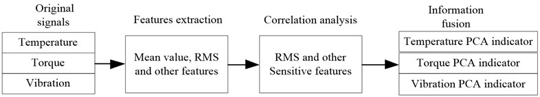
Firstly, after filtering and noise-reduction, a number of features of temperature, torque and vibration signal in time-domain were respectively extracted, such as the maximum, peak-to-peak, variance, root-mean-square, root amplitude, mean, kurtosis, and kurtosis, etc.
Secondly, correlation analysis was used to choose the sensitive features. The correlation coefficients of every feature were gotten according to the Eq. (1):
where represents the correlation coefficient, is a certain feature value of original signal at th moment, is the original signal at th moment, is the mean of , is the mean of , is the total number of data points. 0.85 is generally chosen as the coefficient threshold [20], which indicates that the feature is sensitive to the condition changes of slewing bearing when the correlation coefficient is greater than 0.85, and this feature is retained as sensitive feature, or else eliminated.
Finally, sensitive features were used to construct effective performance recession indicators based on PCA method. The original feature matrix is shown in Eq. (2):
where , 1, 2,..., ; is the th feature value at the th moment, 1, 2,..., . Standardization and normalization processing of the original feature matrix is carried out, shown in Eq. (3):
Then according to the PCA theory[27], a linear group was obtained by transforming new comprehensive variables of feature values (see Eq. (4)):
where each of , ,..., is a new constructed vector, and , ,..., are unrelated (9) and variance of them decreases in sequence. is the first principal component, is the second principal component, and so on there are I main components. is principal component coefficient, and 1, 1, 2,..., , 1, 2,..., . And is the eigenvector corresponding to the eigenvalue of the covariance matrix of matrix , and is also the projection coefficient vector of the original variables of principal component . At last, a principal component whose cumulative contribution rate is the greatest was chosen as performance recession indicator because it reflects the change trend of physical signal best. The cumulative contribution rate is expressed as Eq. (5):
Then, three principal components from temperature, torque, and vibration were chosen as performance recession indicators, which are called as temperature PCA indicator , torque PCA indicator and vibration PCA indicator .
2.2. Life forecasting model
References [19-26] have presented a variety of residual life evaluation methods used to forecast the residual life based on artificial intelligent. But all researchers just made use of some features of vibration as the indicators. Because slewing bearing is a large low-speed heavy-load bearing, vibration signal is insufficient. On the other hand, because of the influence of the environment, it is difficult to obtain failure data of slewing bearing under actual working conditions, and tests also will entails high costs, so that the failure data is limit. Thus, how to establish an effective model with the limit data samples is important to forecast slewing bearing residual life accurately. SVR which specifically gives a solution of the forecasting problem based on small samples is a kind of machine learning algorithm, which has proven highly efficient in life prediction and fault diagnose [19, 20]. In conclusion, this paper proposed a kind of residual life prediction model of slewing bearing, based on SVR method and multiple physical signals, shown in Fig. 2.
Fig. 2Residual life prediction model of slewing bearing
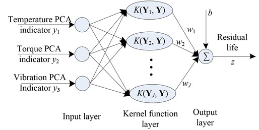
According to Eqs. (4-5), temperature PCA indicator , torque PCA indicator and vibration PCA indicator were selected as three inputs of life model, and life is the output of residual life prediction model. There is a non-linear relationship between the indicators and residual life of slewing bearing. Kernel function was introduced to the SVR algorithms in order to map the input data to high-dimensional feature space (Hilbert space). Then the nonlinear problem was transformed to a linear one. is the kernel functions in the SVR, is the weight vector, 1, 2,…, , and . Therefore, the relationship between indicators and life at the th moment is as following Eq. (6):
where is the threshold value, 1, 2,..., .
The kernel functions are divided into the global kernel functions represented by polynomial and local kernel functions represented by radial basis function (RBF). Different types of Kernel functions have less influence on the predictive ability of SVR [30]. Since RBF can replace the polynomial and has some advantages of few parameters and simple calculation [28], then the following RBF was selected as the kernel function:
where is recognized as the squared Euclidean distance between and , is a traditional deviation used to limit the radial effect range of kernel function which is optimized by particle swarm optimization (PSO) described in Section 2.3, is the center of kernel function which are chosen randomly in the input sample datum. The SVR basic model was used in this paper [29], the following function was used to fit the training datum:
where is the real residual life, and are relaxation factors, is the insensitive factor. So the weight vector and the threshold value can be obtained by solving the optimal target function below combining Eq. (8):
where is a penalty factor which is a constant which is which is optimized by PSO described in Section 2.3. And the result of the model was assessed by root mean square error (RMSE):
where is the prediction value.
2.3. Parameters Optimization of SVR
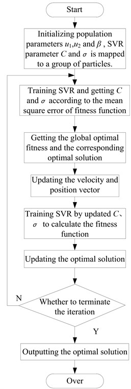
Different types of Kernel functions have less influence on the predictive ability of SVR, however, the traditional deviation of kernel function and penalty factor of the optimal target function have great influence on the prediction performance of SVR, so it is necessary to select appropriate parameters and to improve the prediction ability of SVR [30]. The common and good optimization algorithms include grid optimization (GO), particle swarm optimization (PSO) and genetic algorithm (GA) [31]. After performance comparing, PSO was chosen to optimize the key parameters of SVR. The specific steps of optimizing SVR internal parameters by PSO are shown in Fig. 3, followed by initializing population parameters to train SVR, getting and according to the mean square error of fitness function, getting the global optimal fitness and the corresponding optimal solution, then training SVR by constantly updating the velocity and position vector and getting the optimal solution continuously until compliance with iteration termination conditions, outputting the corresponding optimal solution to train SVR prediction model, inputting signal into the trained model and outputting prediction value at last. According to reference [30], the population parameters 1.49, 0.1, iterations are limited within 200, prediction err of fitness function is within 0.01.
Fig. 3Parameters optimization of SVR based on PSO
3. Real cases and data acquisition
3.1. Slewing bearing test-rig and life test
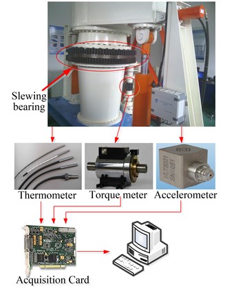
In order to evaluate the new strategy based on multiple physical signals mentioned above, an accelerate fatigue life test was carried out using a special slewing bearing test-rig as shown in Fig. 4. The test sample is a slewing bearing with the raceway diameter of 1 meter and the fatigue carrying capacity of 240 kNm overturning moment and 96 kN axial load, and the rotate speed is 4 rpm. Thermometer is installed in the oiling hole of the slewing bearing to detect the working temperature of raceway. Torque meter is installed in the driver to detect the friction torque of slewing bearing. Accelerometer is attached on the slewing bearing surface to measure the vibration. The signals collected by NI DAQ Card (Data Acquisition Card) are transmitted to a computer through PCI bus. The signal storage and handling are implemented by LabVIEW software.
Fig. 4Accelerated fatigue life test-rig for slewing bearing
In the fatigue life test, the loads increased by 25 %, 50 %, 75 %, 100 % of the fatigue carrying capacity step by step. Loading order and the load values are shown in Table 1. Firstly, slewing bearing rotated at the speed of 4 rpm with 25 % of fatigue carrying capacity. After 30 minutes, the loads were increased to 50 % of fatigue carrying capacity. After 60 minutes, the loads were increased to 50 % of fatigue carrying capacity. After 240 minutes, the loads were increased to full loads, and the slewing bearing continuously rotated until failure.
Table 1Loading order and the values of various forces
Percent of full loads | Turnover moment (kNm) | Axial force (kN) | Speed (rpm) | Duration (minute) |
25 % | 60 | 24 | 4 | 30 |
50 % | 120 | 48 | 4 | 60 |
75 % | 180 | 72 | 4 | 240 |
100 % | 240 | 96 | 4 | Continuously failure |
The test stopped when the slewing bearing got stuck and come to a critical failure after 10.5 days, and the damaged out ring, inner ring, the retainer and the ball after the test are shown in Fig. 5. It can be observed that the outer (fixed) ring raceway is seriously worn, and there are many fatigue spalls around the raceway. On the contrary, there are only a few dents and pitting around the inner (rotatable) ring raceway. Many of the balls and retainers are cracked or even fractured.
Fig. 5The damage of the slewing bearing parts after the test

a) The inner ring
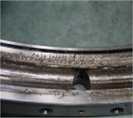
b) The outer ring
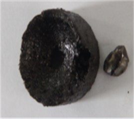
c) The retainer

d) The steel ball
3.2. Data acquisition
The test-rig adopts three kinds of sensors. Thermometer detects the working temperature of slewing bearing raceway. Torque meter detects the friction torque of slewing bearing. Accelerometer measures the vibration of slewing bearing. The original temperature, torque and vibration signals for analysis subsequently are as shown in Fig. 6.
Fig. 6(a), the temperature differs in the day from in the night, so the temperature curve fluctuates. The temperature curve rises slowly before 1000th point, and keeps balanced between the 1000th point and 2200th point, so the period between 0th and 2200th point is called the slewing bearing normal working period. Temperature rises after 2200th point, and rises sharply after 2500th point and reaches a decline period between 2200th and 2640th. At the 2640th point, the temperature rises up to 38 degrees, the slewing bearing gets into the failure period. At last the slewing bearing was stuck and unable to be operated. Fig. 6(b), it is similar to the analysis of temperature signal, the torque signal can also be classified as normal working period, decline period and failure period. The torque rises sharply in decline period due to fault occurs and declines in failure period. This is consistent with the trends of temperature. Fig. 6(c), because of the influence of the background noise, the change of the vibration signal is not obvious, but continued to show an increasing trend in normal running period. It rises in decline period and intensifies in failure period.
4. Model verification and analysis
4.1. PCA indicators
The life test data of slewing bearing introduced in Section 3.2 was used to analyze and verify the residual life prediction model proposed in this paper. Selection and extraction of performance recession indicators are based on the life cycle of the signal trend as the evaluation criteria. Firstly, the PCA indicators were selected that can reflect the residual life trends of slewing bearing. The features and their expressions of original signals are also shown in Table 2. And according to the Eq. (1), the correlation coefficients were obtained.
Fig. 6The original temperature, torque and vibration signals
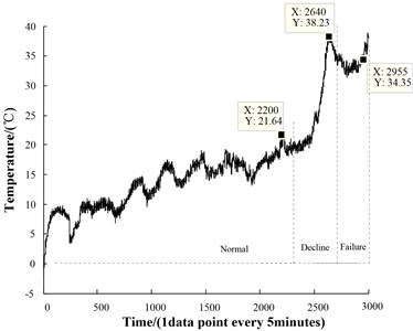
a) The original temperature signal
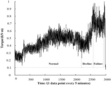
b) The original torque signal
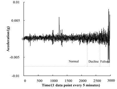
c) The original vibration signal
(1) The maximum, peak-to-peak, variance, root-mean-square, root amplitude, mean, kurtosis, kurtosis value and impulse factor whose correlation coefficient is greater than 0.85 were selected as sensitive features of temperature. data matrix could be obtained by Eq. (2), and then it was normalized in accordance with [0, 2] by Eq. (3). The principal component coefficient matrix was composed of the feature vectors corresponding to the eigenvalues of the covariance matrix . And the 93.6178 % cumulative contribution rate of the first principal component obtained by Eq. (5) exceeded 85 %, so equaled 1. Temperature PCA performance recession indicator for each point of time is shown in Fig. 7. Compared with the original signal Fig. 6(a), it can not only show natural temperature rising process, but also capture the rapid changes sensitively (a sharp rising at the 2500th point). The change of temperature PCA indicator is consistent with the one from slow to fast decrease in the natural state of the life cycle. So these 9 sensitive features selected in this paper can accurately reflect the performance recession trend of slewing bearing.
(2) The maximum, peak-to-peak, variance, kurtosis value, impulse factor and clearance factor were selected as sensitive features of torque. And the 88.4822 % (>85 %) cumulative contribution rate of the first principal component was obtained by Eq. (5), similar to the temperature signal analysis process, also equaled 1. Torque PCA performance recession indicator is shown in Fig. 8. Compared with the original signal Fig. 6(b), the volatility is small. It shows obvious trends at 2500 point. Torque PCA indicator better reflects the performance recession evolution trend of slewing bearing and is consistent with the temperature PCA indicator trends. Therefore, the torque PCA indicator was selected as one of the inputs of the residual life model.
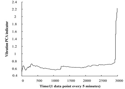
(3) The kurtosis, mean, root-mean-square, root amplitude, shape factor and clearance factor are selected as sensitive features of vibration. And the 85.3834 % (>85 %) cumulative contribution rate of the first principal component was obtained by Eq. (5), and was also 1. Vibration PCA performance recession indicator is shown in Fig. 9. The trend is consistent with the original signal. Vibration is the common signal for data based diagnosis or life prediction. Therefore, the vibration PCA indicator was selected one of the inputs of the residual life model.
Fig. 7Temperature PCA index curve
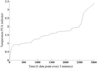
Fig. 8Torque PCA indicator
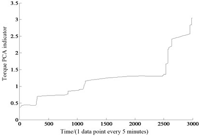
Table 2The features and their correlation coefficients
Features | Expressions | Correlation coefficients | ||
Temperature | Torque | Vibration | ||
Maximum | 0.91 | 0.91 | 0.87 | |
Peak-to-peak | 0.90 | 0.90 | 0.82 | |
Variance | 0.89 | 0.87 | 0.86 | |
Root-mean-square | 0.91 | 0.81 | 1 | |
Root amplitude | 0.88 | 0.79 | 0.72 | |
Mean | 0.89 | 0.80 | 0.89 | |
Kurtosis | 0.90 | 0.78 | 0.58 | |
Shape factor | 0.44 | 0.83 | 0.89 | |
Kurtosis value | 0.92 | 0.85 | 0.89 | |
Impulse factor | 0.90 | 0.86 | 0.88 | |
Clearance factor | 0.84 | 0.86 | 0.77 | |
Fig. 9Vibration PCA indicator
4.2. Performance discussion of models based on different physical signals
Through the above analysis, three effective performance recession quantitative indicators were constructed. Its relationship with the slewing bearing residual life evaluation will be explored according to Section 2.2. To verify the advantages of multiple physical signals based model, seven different models are built base on three single signals, three groups of double signals and a group of three signals respectively. According to the test, 100 sets of data are used to train the model and the 50 sets of data selected randomly are used to test the model. Using the particle swarm optimization, the best traditional deviation of kernel function is 2.25, the best penalty factor of the optimal target function is 85.317. Actual residual life minus forecast value is the error. Fig. 10 shows errors of different models. The correlation coefficients of the forecasting and actual curve are obtained based on Eq. (1), RMSEs are obtained based on Eq. (10). And both of them are used to evaluate the model, as shown in Table 3.
Fig. 10The prediction error of different models
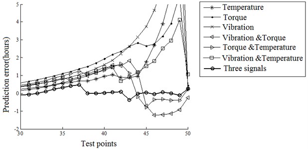
Table 3The comparison of evaluation errors of different models
PCA indicators input into model | Correlation coefficients | RMSEs | |
Single signal | Temperature | 0.851574 | 0.105673 |
Torque | 0.798573 | 0.128003 | |
Vibration | 0.677546 | 0.187139 | |
Double signals | Temperature, torque | 0.863295 | 0.049636 |
Temperature, vibration | 0.840829 | 0.090365 | |
Torque, vibration | 0.945045 | 0.0193599 | |
Three signals | Temperature, torque and vibration | 0.987198 | 0.00445101 |
Fig. 10 shows evaluation effect of life models based on the single signal, double signals and three signals. The prediction errors decrease with the number of signals increases. The single signal based life model is most affected by the historical data, while the multiple signals based model avoids this influence, and the prediction effect is better. According to Table 3, the single signal based RMSE reaches up to 0.187, the double signals based RMSE gets a marked decline, and the three signals based RMSE is just 0.004. The multiple signals based model makes the full consideration of the influence among the temperature, torque and vibration and makes the best of the test data.
4.3. Verification of the complete life prediction model
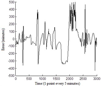
There, this paper used the temperature PCA indicator, torque PCA indicator and vibration PCA recession indicator as input to build the residual life prediction model of slewing bearing. There were 3000 groups of data, 2000 groups were chosen as the training sets and the remaining 1000 groups act as test sets randomly. The mapping relationship between PCA performance recession indicator and residual life were obtained, as shown in Fig. 11. The correlation coefficient of the life model evaluation result is 99.3762 %, which illustrates that multiple signals based life prediction model has good predictive effect. And the errors of real residual life and prediction life at every point are shown in Fig. 12. The RMSE is 0.00214895 which shows that the prediction life is more close to the real life. The result shows that the proposed method can be used in the life prediction of slewing bearing.
Fig. 11Comparison of real residual life and prediction life
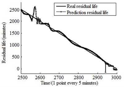
Fig. 12The errors between real residual life and prediction life
5. Conclusion
This paper proposes a multiple physical signals based residual life prediction model. The results have indicated that (1) PCA fusion combined correlation based features selection is an effective method of choosing the performance regression indicators, which is able to make full use of various features. (2) The residual life prediction model based on temperature, torque and vibration signals can well reflect the performance recession trend of slewing bearing and is suitable to predict the residual life effectively.
References
-
Zupan S., Prebil I. Carrying angle and carrying capacity of a large single row ball bearing as a function of geometry parameters of the rolling contact and the supporting structure stiffness. Mechanism and Machine Theory, Vol. 36, Issue 10, 2001, p. 1087-1103.
-
Ignacio Amasorrain Jose, Sagartzazu Xabier, Damian Jorge Load distribution in a four contact-point slewing bearing. Mechanism and Machine Theory, Vol. 38, Issue 6, 2003, p. 479-496.
-
Kunc Robert, Prebil Ivan Numerical determination of carrying of large rolling bearings. Journal of Materials Processing Technology, Vols. 155-156, 2004, p. 1696-1703.
-
Kunc Robert, Zerovnik Andrej, Prebil Ivan Verification of numerical determination of carrying capacity of large rolling bearings with hardened raceway. International Journal of Fatigue, Vol. 29, 2007, p. 1913-1919.
-
Daidie Alain, Chaib Zouhair, Ghosn Antoine 3D simplified finite elements analysis of load and contact angle in a slewing ball Bearing. Journal of Mechanical Design, Vol. 130, 2008, p. 1-8.
-
Gao Xuehai, Huang Xiaodiao, Wang Hua Effect of raceway geometry parameters on the carrying capability and the service life of a four-point-contact slewing bearing. Journal of Mechanical Science and Technology, Vol. 24, Issue 10, 2010, p. 2083-2089.
-
Potocnik Rok, Goencz Peter, Glodez Srecko Static capacity of a large double row slewing ball bearing with predefined irregular geometry. Mechanism and Machine Theory, Vol. 64, Issue 1, 2013, p. 67-79.
-
Wang Yanshuang, Cao Jiawei Determination of the precise static load-carrying capacity of pitchbearings based on static models considering clearance. International Journal of Mechanical Sciences, Vol. 100, 2015, p. 209-215.
-
Kim Hack-Eun, Tan Andy C. C., Mathew Joseph, Choi Byeong-Keun Bearing fault prognosis based on health state probability estimation. Expert Systems with Applications, Vol. 39, 2012, p. 5200-5213.
-
Caesarendra Widodo A., Thom P. H., Yang B. S., Setiawan J. D. Combined Probability approach and indirect data-driven method for bearing degradation prognostics. IEEE Transactions on Reliability, Vol. 60, Issue 1, 2011, p. 14-20.
-
Lei Yaguo, He Zhengjia, Zi Yanyang A combination of WKNN to fault diagnosis of rolling element bearings. Journal of Vibration and Acoustics, Vol. 131, Issue 6, 2009, p. 064502.
-
Widodo A., Yang B. S. Machine health prognostics using survival probability and support vector machine. Expert Systems with Applications, Vol. 38, 2011, p. 8430-8437.
-
Moodie C. A. S. An investigation into the condition monitoring of large slow speed slew bearings. Ph.D. Thesis, University of Wollongong, Wollongong, 2009.
-
Wahyu Caesarendra, Prabuono Buyung Kosasih, Anh Kiet Tieu, Craig Alexander Simpson Moodie, Byeong-Keun Choi Condition monitoring of naturally damaged slow speed slewing bearing based on ensemble empirical mode decomposition. Journal of Mechanical Science and Technology, Vol. 27, Issue 8, 2013, p. 2253-2262.
-
Ye Yixi, Xiao Hanbin Extraction of vibration signal of large-scale bearing based on wavelet analysis. Journal of Wuhan University of Technology, Vol. 28, Issue 6, 2008, p. 840-843.
-
Zvokelj M., Zupan S., Prebil I. Multivariate and multiscale monitoring of large-size low-speed bearings using ensemble empirical mode decomposition method combined with principal component analysis. Mechanical Systems and Signal Processing, Vol. 24, Issue 4, 2010, p. 1049-1067.
-
Zvokelj M., Zupan S., Prebil I. Non-linear multivariate and multiscale monitoring and signal denoising strategy using kernel principal component analysis combined with ensemble empirical mode decomposition method. Mechanical Systems and Signal Processing, Vol. 25, Issue 7, 2011, p. 2631-2653.
-
Wahyu Caesarendra, Buyung Kosasih, Anh Kiet Tieu, Craig Alexander Simpson Moodie Circular domain features based condition monitoring for low speed slewing bearing. Mechanical Systems and Signal Processing, Vol. 45, 2014, p. 114-138.
-
Benkedjouh T., Medjaher K., Zerhouni N., Rechak S. Remaining useful life estimation based on nonlinear feature reduction and support vector regression. Engineering Application of Artificial Intelligence, Vol. 26, 2013, p. 1751-1760.
-
Shen Zhongjie, Chen Xuefeng, He Zhengjia, et al. Remaining life predictions of rolling bearing based on relative features and multivariable support vector machine. Journal of Mechanical Engineering, Vol. 49, Issue 2, 2013, p. 183-189.
-
Xi Lifeng, Huang Runqing, Li Xinglin, et al. Residual life predictions for ball bearing based on neural networks. Chinese Journal of Mechanical Engineering, Vol. 1, 2007, p. 193-207.
-
Sikorska J. Z., Hodkiewicz And Ma M. L. Prognostic modeling options for remaining useful life estimation by industry. Mechanical Systems and Signal Processing, Vol. 25, Issue 5, 2011, p. 1803-1836.
-
Gebraeel N., Lawley M., Liu R., et al. Residual life predictions from vibration-based recession signals: a neural network approach. IEEE Transactions on Industrial Electronics, Vol. 51, 2004, p. 694-700.
-
Cong F. Y., Chen J., Pan Y. N. Kolmogorov-Smirnov test for rolling bearing performance recession assessment and prognosis. Journal of Vibration and Control, Vol. 17, Issue 9, 2011, p. 1337-1347.
-
Wang H. W., Wu H. Q. Residual useful life prediction for aircraft engine based on information fusion. Journal of Aerospace Power, Vol. 27, Issue 12, 2012, p. 2749-2755.
-
Benkedjouh T., Medjaher K., Zerhouni N., et al. Remaining useful life estimation based on nonlinear feature reduction and support vector regression. Engineering Applications of Artificial Intelligence, Vol. 26, Issue 7, 2013, p. 1751-1760.
-
Abdi H., Williams L. J. Principal component analysis. Wiley Interdisciplinary Reviews: Computational Statistics, Vol. 2, Issue 4, 2010, p. 433-459.
-
Ayata N. E., Cherieta M., Suenb C. Y. Automatic model selection for the optimization of SVM kernels. Pattern Recognition, Vol. 38, 2005, p. 1733-1745.
-
Vapnik V. N. Statistical Learning Theory. Wiley, New York, 1999.
-
Zhang N. Research on the Parameter Optimization of SVR. Northwestern Polytechnical University, Xian, 2008.
-
Li Y. Y. Research on Group Intelligent Optimization Based on SVM. Tianjing University, Tianjing, 2007.
Cited by
About this article

The authors gratefully acknowledge the support provided by the National Natural Science Foundation of China (51105191, 51375222), the Shanghai Sailing Program (16YF1408500) and China Postdoctoral Science Foundation (Project No. 2015M580632).
