Abstract
In this paper energy harvesting from vibrating surfaces through electromagnetic induction is addressed. A double pendulum subject to base excitations generates electrical energy through energy harvesting coils mounted on the pendulum masses. Optimum double pendulum generates energy at a rate of 9 mW for excitation parameters characteristic of bridge vibration, frequency of 2 Hz and amplitude of 1 mm.
1. Introduction
Energy harvesting is a process of transforming ambient vibrational kinetic energy into useful electrical energy to power devices and sensors with modest energy requirements. If implemented successfully, it can save time and costs required to maintain the batteries currently being used to power sensors.
Systems in which the force of excitation depends the upon a system parameter are called parametrically excited systems. Rand in [1], discusses the most basic parametrically excited system, Mathieu equation. It is shown that the amplitude of oscillation of pendulum grows exponentially when the forcing frequency is twice the natural frequency of the pendulum. Jial and Seshia in [4] show unlike the linear resonance, oscillatory amplitude growth in parametric resonance is not limited by linear damping. Zaghari, et al. in [2] showed that a small excitation can produce a large response when the system is parametrically excited with a frequency near to twice of its fundamental frequency. Krzysztof Kecik [3] proposed conception of simultaneous elimination of vibration and energy induction by a pendulum motion. Michal Marszal et al in [6] derived the double pendulum natural frequency for the out-of-phase and in-phase modes. A. C. Skeldon explored parametrically excited double pendulum in [5] found a range of complicated dynamical phenomena in a region where the excitation frequency was close to twice the natural frequency. The work presented aims at harvesting energy by harnessing the advantages offered by autoparametric resonance.
2. Double pendulum governing equation
The double pendulum is the simplest mechanical apparatus that exhibits a range of dynamic responses from periodic oscillations to chaotic rotations. This utility can be harnessed to maximize harvest energy from a double pendulum subject to base excitation.
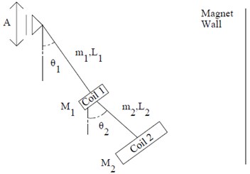
Consider the double pendulum shown in Fig. 1. Let the two pendulum lengths be and . The pendulum masses are cylindrical coils of radius and masses and and pendulum link masses and . The generalized co-ordinates for the double pendulum system are the angles made by the two pendulum links with the vertical, and . The double pendulum is excited by surface vibrations with amplitude and frequency . The governing equation of motion for a dissipative system can be derived using the Euler-Lagrangian equation given by:
where, Lagrangian function, is the difference between the system kinetic energy and potential energy, , is the Rayleigh dissipation function and is the system generalized coordinate. The system kinetic energy, , is obtained by differentiating mass co-ordinates with time:
Fig. 1Schematic of an energy harvesting double pendulum subject to base excitation facing a magnet wall
Potential energy of the system assigning pivot point zero potential energy reference is given by:
Frictional torque at the bearing as given in reference [8] is given by, , where, is the coefficient of friction, is the bearing bore diameter and is the dynamic radial load on the bearing. The Rayleigh dissipation function for frictional damping:
Viscous air drag on the coil is approximated as the viscous force acting on a sphere of the same radius. The air drag force acting on a sphere of radius , moving with a velocity , is given by, , where, is dynamic coefficient of viscosity, 2e-5 kg/ms for air. Substituting 12.56e-7, the Rayleigh dissipation function to incorporate viscous losses:
Power harvested by induced electromagnetic voltage is given by the equation, , where, is the number of loops in the coil, is the magnetic field strength, is the area of enclosed by each coil, is the angle between the normal to the coil area vector and magnetic field lines, is the coil resistance. Taking , Rayleigh dissipation function for electromagnetic damping:
Total Rayleigh function, . Following constants are substituted for the corresponding ratios to non-dimensionalize expressions and simplify notation:
Non-dimensional equations governing the two degrees of freedom and are given by:
3. Numerical simulations
A standard copper coil with dimensions and wire properties listed in Table 1 is taken as pendulum one mass . Working out the electromagnetic damping coefficient and mass from the dimensions gives us, 0.00056 kg/s and 1.6 kg. Since the coil is massive, the ratio link mass to coil mass can be approximated to zero, 0.
Natural frequency of the double pendulum for small oscillation amplitudes is obtained by implementing method of harmonic balance as employed by Roy et. al in [7]. Neglecting damping and forcing in Eqs. (7-8), the equations reduce to:
Trigonometric ratios sine and cosine are expanded to first two terms. Substituting and where is the natural frequency of double pendulum, higher powers of trigonometric ratios are expanded as linear combinations of higher harmonics. Coefficient of in the resulting equations is equated to zero to remove secular terms to obtain:
Table 1Standard coil dimensions
Coil ID | Coil OD | Wire diameter () | Turns () | Resistivity () | Wire density () | Magnetic field () |
23 mm | 40 mm | 1.4 mm | 1100 | 1.7e-9 Ω/m2 | 8900 kg/m3 | 0.01 T/m2 |
Eqs. (11-12) are treated as two linear conditions on the amplitude of oscillation and , and for consistency demand that:
When solved for frequency, , two solutions obtained correspond to in-phase oscillation , and out-of-phase oscillation , . In-line with the small angles of oscillation assumption, substituting 0.3 in Eq. (13), natural frequencies of the two modes of oscillation:
In Fig. 3, energy harvested is plotted against the frequency ratio, /for in-phase and / for out-of-phase oscillating double pendulum. Pendulum length, is changed to satisfy the forcing frequency to natural frequency ratio, , according to:
Distinct energy peak is seen at frequency ratio 2 in both Figs. 2(a) and 2(b) for the two modes of oscillation. The analysis below, attempts to identify optimum and to harvest maximum energy from a source vibrating with fixed amplitude and frequency. The autoparametrically resonant pendulum link length, , is modified as and vary according to Eq. (15) for 2. In the Fig. 3(a) and 3(b) energy harvested in 100 seconds for steady state oscillations is plotted along the -axis for in-phase and out-of-phase oscillations respectively. and vary over the domain, 0.1, 2.5.
Fig. 2Energy harvested in 100 seconds, 1 <n< 5 for two modes of oscillation, a= 1, b= 1, A= 1 mm, Ω= 10π rad/s
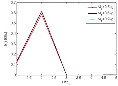
a) In-phase oscillation
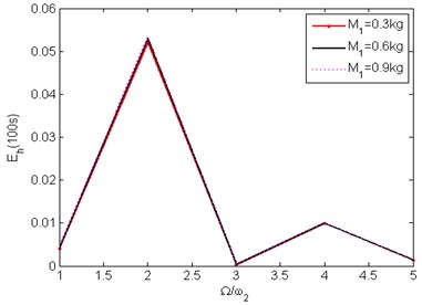
b) Out-of-phase oscillation
Fig. 3Energy harvested in 100 seconds by autoparametrically resonant double pendulum over the a-b domain, A= 1 mm, Ω= 10π rad/s
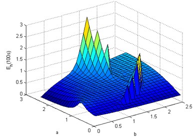
a)2
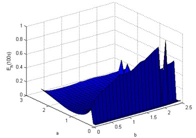
b)2
The ideal energy harvester, optimum autoparametric in-phase oscillating double pendulum cannot be realized for practical implementation as seen readily by the dimensions given in Table 2. The resonant out-of-phase oscillating double pendulum is a more pragmatic alternative.
Table 2Dimension of optimum double pendulum for the two modes of oscillation
Power | |||||
1.25 cm | 1.6 kg | 3.75 cm | 2.24 kg | 30 mW | |
31 cm | 1.6 kg | 10 cm | 3.5 kg | 9 mW |
Fig. 4Energy harvested in 100 seconds by double pendulum with optimal a and b for the two modes of oscillation over realisable L1
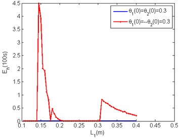
Amplitude of in-phase oscillation of the two angles, and , for practically realizable link lengths decays harvesting negligible steady state energy as seen by the blue plot in Fig. 4. In-case of out-of-phase initial conditions (red plot in Fig. 4) plot rises exactly at autoparametrically resonant 31 cm, generating 9 mW in steady state validating importance of autoparametric resonance. The peak at 15 cm corresponds to out-of-phase 1:4 resonance. Maximizing energy harvested requires a comprehensive study of such variety of responses, especially so for high frequency base excitation where attaining resonance entails an even shorter pendulum link length.
4. Conclusions
The in-phase oscillating pendulum harvests energy at a rate of 30 mW, more than five times that of an equivalent autoparametrically resonant simple pendulum, for modest excitation parameters, 1 mm, 10 rad/s. Pendulum one link length obtained for in-phase resonance is too short for practical implementation. While, the optimum out-of-phase oscillating double pendulum, harvests energy at 9mW, which might just be sufficient to power maintenance sensors, the dimensions obtained for double pendulum are realizable, making out-of-phase oscillation a more desirable mode of oscillation for energy harvesting. Application specific design may help design by adding constrains on more equation parameters, which can help us in optimizing the remaining parameters more comprehensively giving better results.
References
-
Rand Richard http://www.math.cornell.edu/rand/randdocs/nlvibe52.pdf, 2016.
-
Zaghari B., Tehrani M. Ghandchi, Rustighi E. Mechanical modeling of a vibration energy harvester with time-varying stiffness. 9th International Conference on Structural Dynamics, 2014, p. 2079-2085.
-
Kecik K., Borowiec M. An autoparametric energy harvester. European Physical Journal Special Topics, Vol. 222, 2013, p. 1597-1605.
-
Jia Y., Seshia A. A. A parametrically excited vibration energy harvester. Journal of Intelligent Material Systems and Structures, Vol. 25, Issue 3, 2014, p. 278-289.
-
Jia Y., Seshia A. A. Directly and parametrically excited bi-stable vibration energy harvester for bistable operation. 17th International Conference on Solid-State Sensors, Actuators and Microsystems (Transducers and Eurosensors), 2013, p. 454-457.
-
Marszal Michal, Jankowski Krzysztof, Perlikowski Przemyslaw, Kapitaniak Tomasz Bifurcations of oscillatory and rotational solutions of double pendulum with parametric vertical excitation. Mathematical Problems in Engineering, Vol. 2014, 2014, p. 892793.
-
Roy Jyotirmoy, Mallik Asok K., Bhattacharjee Jayanta K. Role of initial conditions in the dynamics of a double pendulum at low energies. Nonlinear Dynamics, Vol. 73, 2013, p. 993-1004.
-
www.roymech.co.uk/UsefulTables/Tribology/Bearing.html, 2016.
About this article

