The analysis of the ventricle assist device controlled rotor dynamics

Ovsyannikova, Elena; Gouskov, Alexander M.

Vibroengineering Procedia

Browse Procedia

Published: 07 October 2016

Check for updates

The analysis of the ventricle assist device controlled rotor dynamics

Elena Ovsyannikova¹

Alexander M. Gouskov²

^{1, 2}Moscow Bauman State Technical University, Moscow, Russia

Corresponding Author:

Alexander M. Gouskov

Cite the article Download PDF

Downloads 1331

Abstract

The analysis of dynamics of rotor-driven artificial ventricle (VAD) was conducted in the work. A comparison of two types of control is given: a linear-quadratic (LC) optimization and PID-regulator. It was shown that LC – control allows the pump rotor positioning with an accuracy of 0.2 mm at speeds ranging from 5,000 to 12,000 rev/min.

1. Introduction

The problems of heart failure are particularly acute in recent years. One of the variants of solution became circulatory support devices –ventricle assist devices (VADs). In accordance with articles [1-3], the axial VADs are preferred nowadays. The work is devoted to describing the VAD rotor dynamics: the theoretical bases were shown; the equation of motion was obtained; active magnetic bearings were considered. The question of the rotor movement control was considered: two types of control were selected for comparison, PID control and LC-management. The numerical simulation of the rotor stabilization was realized. The rotor positioning error had not to exceed 0.2 mm. The behavior of the rotor and the control response is examined in the speed range from 5000 rev/min to 12000 rev/min.

2. Statement

The symmetric homogeneous rigid rotor rotating along the longitudinal axis at a constant angular velocity in two radial active magnetic bearings AMP1 (A) and AMP2 (B) of axial pump VAD is considered. Specifications are given in the tables (Table 1).

Table 1Rotor technical characteristics

Nomination	Symbol	Value
Diameter, m	$D$	15.6×10^-3
Length, m	$l$	24×10^-3
Mass, kg	$m$	12.42×10^-3
Positioning accuracy, mm	$ε$	≤ 0.2
Rotation frequency, rev./min.	$Ω$	5000-12000
Length from rotor center mass to bearings, m	$a$	9×10^-3
Length from rotor center mass to bearings, m	$b$	9×10^-3
Length from rotor center mass to censors, m	$c$	10×10^-3
Length from rotor center mass to censors, m	$d$	10×10^-3

The assumptions for the equation of motion are the following [4]:

1) The rotor is symmetric and rigid.

2) Deviations from the reference position are small in comparison with the rotor dimensions.

3) The angular velocity $Ω$ of the rotor about its longitudinal axis $z$ is assumed tobe constant.

The inclinations and the angular motion around the rotor spin axis are described by the three so-called Cardan angles $α$ , $β$ , $γ$ . Linearization leads to characterizing the angles $α$ , $β$ as inclinations about the $X$ and $Y .$ The equations of motion are given for the variables $q = {\{β, x_{S}, - α, y_{S}\}}^{T}$ .

3. Model and equation of motion

The equations of motion follow from Lagrange’s equations:

1

\frac{d}{d t} (\frac{\partial T}{\partial {\dot{q}}_{i}}) - \frac{\partial T}{\partial q_{i}} = Q_{i}, i = 1 . . . 4,

with the kinetic energy $T$ and generalized forces $Q_{i}$ , $q_{i}$ – the generalized coordinates. The kinetic energy $T$ is:

2

T = \frac{1}{2} m ({\dot{x}}_{S}^{2} + {\dot{y}}_{S}^{2} + {\dot{z}}_{S}^{2}) + \frac{1}{2} Ω^{T} Ι_{S} Ω,

where ${\dot{x}}_{S}$ , ${\dot{y}}_{S}$ , ${\dot{z}}_{S}$ – components of center mass velocity, $Ι_{S}$ – rotor inertia tensor $Ω$ – angular velocity vector.

Equation of motion of the rotor with active magnetic bearings [4]:

3

M \ddot{q} (t) + G \dot{q} (t) + K q (t) = B_{q} K_{i} i (t) + F_{e x t},

where $M$ [4×4] – symmetric positive definite mass matrix, $G$ [4×4] - skew-symmetric gyroscopic matrix, $K$ [4×4] – stiffness matrix, $B_{q}$ [4×4] – transformation matrix which relates the generalized coordinates of the rotor center mass to the rotor displacements in magnetic bearings, $K_{i}$ [4×4] – matrix of current stiffness’s, $i (t)$ [4×1] – vector of currents in magnets, $F_{e x t}$ [4×1] – vector of generalized external forces.

The rotor receives the load $F_{e x t}$ as the force of gravity and the moments from the hydrodynamic forces in the fluid flow:

4

F_{e x t} (t) = \{\begin{array}{l} C μ π R^{2} l (- \dot{β} (t) + Ω α (t)), \\ A_{1} c o s (ω t), \\ C μ π R^{2} l (- \dot{α} (t) - Ω β (t)), \\ - m g + A_{2} c o s (ω t), \end{array}

where $μ$ – the blood viscosity, $μ =$ (3-4)×10^-3 Pa∙s at 37 °С, $C$ – the drag coefficient, $C =$ 0,91-0,85, $R$ – radius, $l$ – length, $Ω$ – rotation frequency. The impact of external influences on a person is taken into account in the form of vibration, expressed by harmonic functions, acting at the $x$ and $y$ axes: $A_{1}$ , $A_{2}$ – the amplitudes of the oscillation of transport.

4. Control types

4.1. The decentralized PID-control

The local control shown in Fig. 1 feeds each local sensor signal back to the corresponding bearing control current using the feedback gains [5]. The four output signals $i (t)$ combine in the output vector $q$ :

5

i (t) = - (P q (t) + D \dot{q} (t) + I \int_{t_{0}}^{t_{1}} q (t) d τ),

with $P$ , $D$ , $I$ – the diagonal matrixes of control coefficients. The equation of motion then takes the form:

6

M \ddot{q} (t) + G \dot{q} (t) + K q (t) + K_{C} q (t) + D_{C} \dot{q} (t) + I_{C} \int_{t_{0}}^{t_{1}} q (t) d τ = F_{e x t} (t),

where $K_{C} = B_{q} K_{i} P C$ and $D_{C} = B_{q} K_{i} D C$ are stiffness and damping matrixes respectively and $Ι_{C} = B_{q} K_{i} I C$ – matrix of integral components, $C$ – transformation matrix.

4.2. The linear quadratic method

Linear-quadratic regulator (LQR) – optimal control algorithm based on the idea of minimizing a certain functional [6]. The novelty of this method is based on varying parameters which can be chosen for different types of conditions. Besides, for this type of control the equation of motion will change, because it should be implemented by bearing coordinates:

7

M_{b} {\ddot{q}}_{b} + G_{b} {\dot{q}}_{b} = B_{q} (- K_{S} q_{b} + K_{i} i) + F_{e x t}, M_{b} = M {(B_{q}^{T})}^{- 1}, G_{b} = G {(B_{q}^{T})}^{- 1} .

In the standard form:

8

\dot{z} (t) = A z (t) + B i (t) + C^{*} F_{e x t},

A = [\begin{matrix} 0 & E \\ - M_{b}^{- 1} B_{q} K_{S} & - M_{b}^{- 1} G_{b} \end{matrix}], B = [\begin{matrix} 0 \\ - M_{b}^{- 1} B_{q} K_{i} \end{matrix}], C^{*} = [\begin{matrix} 0 \\ - M_{b}^{- 1} \end{matrix}] .

Formally control problem can be represented as follows [6]. It is required to find a control law $i (t)$ that minimizes the objective function:

9

J (y (t), i (t)) = \int_{0}^{\infty} [z^{T} (t) Q z (t) + ρ i^{T} (t) R i (t)] d t,

where $z (t) = {\{q_{b}^{T} (t) {\dot{q}}_{b}^{T} (t)\}}^{T}$ – is the solution of the system Eq. (9). $Q \in R^{8 \times 8}$ is positive semi-definite and $R \in R^{8 \times 8}$ – positive definite matrixes, respectively, obtained in accordance with Bryson rule [10]. The control law will be found as:

10

i (t) = - K z (t), K = R^{- 1} B^{T} X .

The equation of motion becomes:

11

\dot{z} (t) = A z (t) - B K z (t) + C F_{e x t}, q_{b} = C^{*} z (t) .

5. Modeling based on PID control

The study of rotor oscillations at fixed positional stiffness of bearings for different rotor speeds was conducted. Yellow line shows oscillations at a rotor speed of 5000 rev/min, the purple – at a speed of 10000 rev/min, green – 12000 rev/min.

For a fixed positional stiffness $k_{S} =$ 10⁴N∙m^-1 the results are illustrated with Fig. 1.

6. Modeling based on LQR method

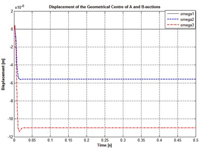
The comparison of the rotor displacements was held at different speeds and constant stiffness. The value of the positional stiffness $k_{S}$ is 10⁵N∙m^-1, of the current stiffness $k_{i}$ – 10 N∙А^-1. The black line shows changes of displacements at 5000 rev/min, blue line – at 10000 rev/min, red line at – 12000 rev/min (Fig. 2).

Table 2Comparison of the displacement amplitude values for different rotation speeds and positional bearing stiffnesses

Rotation speed, rev/min	Max values of displacements $k_{S} =$ 10⁴N×m^-1, m	Max values of displacements $k_{S} =$ 10⁵N×m^-1, m	Max values of displacements $k_{S} =$ 10⁶N×m^-1, m
5000	3.9×10^-7	3.6×10^-7	2.54×10^-7
10000	4.8×10^-7	3.8×10^-7	2.6×10^-7
12000	5.21×10^-7	3.93×10^-7	2.71×10^-7

Fig. 1Displacements of the section centers A and B

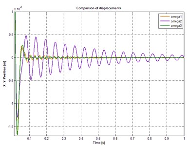
Fig. 2Displacements of the section centers A and B

It can be concluded that with the increase of rotor speed, values of the oscillation amplitudes and of the control currents increase too. However, the obtained values are permissible. The values of currents in the magnets arranged along the $y$ -axis are greater than in magnets along the $x$ -axis. It is due to the fact that in addition to the influence of the hydrodynamic moments of the blood flow the force of gravity acts along the $y$ -axis.

The results obtained for the three types of control have been tabulated (Table 2) for the velocity of 10000 rev/min and 12000 rev/min respectively.

Table 3Comparison of rotor center displacements at different control types at 10000 rev/min. The value of the positional stiffness kS is 105N∙m-1

	PID-control	LQR-method
$x_{b A m a x}$ , m	3.7×10^-7	5.4×10^-7
$y_{b A m a x}$ , m	3.9×10^-7	5.6×10^-7
$i_{b x m a x}$ , mА	5	5.3
$i_{b y m a x}$ , mА	8	5.5

7. Conclusions

The simulation results show that LQR method meets the requirements of the rotor control the best way. It provides the position of the centers of rotor sections within the permissible error – 0.2 mm and allows to optimize the control on several criteria, in this case, criteria were: the position of the bearing section centers and control currents. The results of these studies can be used for real axial pump design.

References

Birks E. J. Left ventricular assist devices. Heart, Vol. 96, 2010, p. 63-71.

Search CrossRef
Thunberg Christopher A., Gaitan Brantley Dollar, Arabia Francisco A., Cole Daniel J., Grigore Alina M. Ventricular assist devices today and tomorrow. Journal of Cardiothoracic and Vascular Anesthesia, Vol. 24, Issue 4, 2010, p. 656-680.

Search CrossRef
Griffith B. P., Kormos R. L., Borovetz H. S., Litwak K., Antaki J. F., Poirier V. L., et al. HeartMate II left ventricular assist system: from concept to first clinical use. The Annals of Thoracic Surgery, Vol. 71, 2001, p. 16-20.

Search CrossRef
Schweizer G., Maslen E. H. Chapter 7: Dynamics of the Rigid Rotorsa; Chapter 10: Dynamics of Flexible Rotors. Magnetic Bearings. Theory, Design and Application to Rotating Machinery, Springer, Berlin Heidelberg, 2009, p. 167-189, p. 251-297.

Search CrossRef
Franklin G. F., Powell J. D., Emami-Naeini A. Feedback Control of Dynamic Systems. 4th Edition. Prentice Hall, Upper Saddle River, NJ, 2002.

Search CrossRef
Barbaraci G., Virzì Mariotti G. Sub-optimal control law for active magnetic bearings suspension. Journal of Control Engineering and Technology, Vol. 2, Issue 1, 2012, p. 1-10.

Search CrossRef

About this article

Received

07 September 2016

Accepted

14 September 2016

Published

07 October 2016

SUBJECTS

Mechanical vibrations and applications

Keywords

mechanical circulatory support

ventricle assist device

artificial heart

active magnetic bearings

dynamics of the control system

LC-control

PID controller

rotor stabilization

Acknowledgements

This work was supported by the Russian Foundation for Basic Research (Grant No. 15-29-01085 ofi_m).

This is an open access article distributed under the Creative Commons Attribution License, which permits unrestricted use, distribution, and reproduction in any medium, provided the original work is properly cited.