Machine learning for rotating machines: simulation, diagnosis and control

1. Introduction

The main tool in modern machine learning is an artificial neural network (ANN) [1]. This work deals with applications of machine learning to rotating machines with fluid-film bearings. A rotor rotation is usually accompanied by lateral vibrations [2, 3]. Rotor trajectory contains information about the condition of the bearings and the rotor machine at a whole. Rotor dynamics modeling is a difficult task especially when the rotor has fluid-film bearings [2]. Hydrodynamic calculations are computationally expensive. Therefore, this part of the rotor dynamics problem can be implemented using ANNs [4]. Modern rotating machines can be equipped with a number of sensors. Analysis of their measurements can be automated using specialized ANNs. These ANNs implement logistic regression [1]. Both shallow learning and deep learning are used in pattern recognition. Deep convolutional neural networks are widely used in fault diagnosis [5, 6]. Deep learning is emerging in reinforcement learning and continuous control systems [7, 8].

This paper unites theoretical and experimental results achieved by the authors in applications of machine learning to simulation, diagnosis and control of rotating machines with fluid-film bearings.

2. Shallow learning for rotor dynamics simulation and fault diagnosis

The goal of supervised learning is to determine relationship between two sets: an input set $\mathbf{X}$ and a target set $\mathbf{Y}$. The difference between predictions $\mathbf{H}$ and targets $\mathbf{Y}$ is minimized in training process. This error function is called a target function, a cost function, or a loss function.

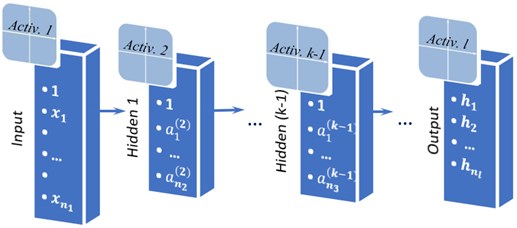
The scheme of a simple feed forward ANN called multilayer perceptron is represented in Fig. 1. The $l$-layer ANN has an input layer, $l-2$ hidden layers and an output layer. A feature of the network architecture is that each neuron of the previous layer transmits its signal to each neuron of the next layer [4].

Input data in the form of $n_1$ numbers can be represented as a one-dimensional matrix. The input layer receives this matrix $\mathbf{X}=\left(\left(x_i^{\left(1\right)}\right)\right)(i=1\dots n_1$) and simply transmits it to the second layer with an additional unit element. The matrix ${\mathbf{A}}^{\left(1\right)}=\left(\left(\begin{array}{cc}1& \mathbf{X}\end{array}\right)\right)$ is the output of the first layer. In the second (hidden) layer data from the first layer is multiplied by the weights matrix ${\text{Θ}}^{\left(1\right)}$ and added ${\mathbf{Z}}^{\left(2\right)}={\mathbf{A}}^{\left(1\right)}{\text{Θ}}^{\left(1\right)}$. An activation function is applied to the result ${\mathbf{Z}}^{\left(2\right)}$, and resulting matrix with additional unit element is the output of the second layer ${\mathbf{A}}^{\left(2\right)}=\left(\left(\begin{array}{cc}1& {activation}^{\left(2\right)}\left({\mathbf{Z}}^{\left(2\right)}\right)\end{array}\right)\right)$. The same actions take place on an arbitrary $k-1$ hidden layer:

where ${\mathbf{Z}}^{(k-1)}$ is matrix with results of multiplication by weights and adding in the current layer, ${\mathbf{A}}^{(k-2)}$, ${\mathbf{A}}^{(k-1)}$ are matrices of outputs in the previous and the current layers respectively, ${\text{Θ}}^{(k-2)}$ is the previous layer weights matrix, ${activation}^{(k-1)}$ is an activation function.

Similar calculations occur in the output layer. The result of the calculation in the output layer is the matrix of predictions $\mathbf{H}=\left(\left({activation}^{\left(l\right)}\left({\mathbf{Z}}^{\left(l\right)}\right)\right)\right)$.

The unknown weights matrices ${\text{Θ}}^{\left(k\right)}$ are determined by minimizing the objective function $J\left({\mathrm{\Theta }}^{\left(k\right)}\right)\Rightarrow min$. The type of objective function depends on the type of a given problem.

Fig. 1An l-layer feed forward neural network with n1 inputs and nl outputs

2.1. Multi-dimensional mapping for rotor dynamics simulation

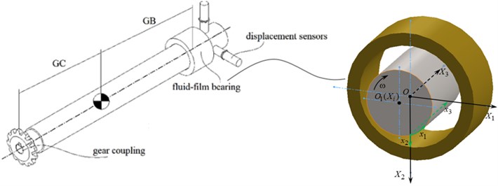
A rigid unbalanced rotor with a gear coupling and a fluid-film bearing at the opposite tips is considered (see Fig. 2). The equations of the rotor’s motion can be represented as follows [3]:

2

$\left\{\begin{array}{l}m{d}^2\mathbf{X}/d{t}^2=\mathbf{C}+\mathbf{B}+\mathbf{F},\\ J_d{d}^2\mathbf{\Psi }/d{t}^2+J_{p}d\mathbf{\Psi }/dt=\mathbf{C}\bullet \mathbf{G}\mathbf{C}+\mathbf{B}\bullet \mathbf{G}\mathbf{B},\end{array}\right.$

where $m$ is rotor mass, $\mathbf{X}$,$\mathrm{}\mathbf{\Psi }$ are coordinates of the center of mass and angles of the rotor rotation respectively, $t$ is time, $\mathbf{C}$, $\mathbf{B}$ are reaction forces of the gear coupling and the bearing respectively, $\mathbf{F}=m\mathrm{\Delta }{\omega }^2\left[\left[\begin{array}{c}\mathrm{c}\mathrm{o}\mathrm{s}(\omega t+\phi )\\ \mathrm{s}\mathrm{i}\mathrm{n}(\omega t+\phi )\end{array}\right]\right]$ is inertia force, $m\mathrm{\Delta }$ is the rotor unbalance, $\phi$ is phase of unbalance, $J_p$, $J_d$ are polar and diametral moments of inertia respectively, $\mathbf{G}\mathbf{C}$, $\mathbf{G}\mathbf{B}$ are radius-vectors to the coupling and to the bearing respectively.

It is assumed that reaction forces are equivalent to springs and dampers: $\mathbf{C}=\mathbf{C}\left(\mathbf{X},d\mathbf{X}/dt\right)$, $\mathbf{B}=\mathbf{B}\left(\mathbf{X},d\mathbf{X}/dt\right)$. Also, it is assumed that reaction in a coupling is linear with given linear coefficients and reaction in a bearing is non-linear. Calculation of the bearing reaction is connected with solution of the Reynolds equation [2, 4]:

3

$\frac{\partial }{\partial x_1}\left[\frac{h^3}{\mu }\frac{\partial p}{\partial x_1}\right]+\frac{\partial }{\partial x_3}\left[\frac{h^3}{\mu }\frac{\partial p}{\partial x_3}\right]=6\frac{\partial }{\partial x_1}\left(u_{1}h\right)-12u_2,$

where $x_i$ are coordinates connected with the thin oil film, $p=p(x_1,x_3)$ is the unknown pressure function, $h=h\left(x_1\right)$ is the oil film thickness, $\mu$ is viscosity, $u_j=u_j\left(x_1\right)$ are the tangential and normal components of the journal surface velocity, where $i=1,2,3$, $j=\mathrm{1,2}$.

Fig. 2Calculation schematic of a rotor-bearing test rig with a fluid-film bearing

Given the pressure function, the components of reaction can be calculated by integration:

4

$\begin{array}{cc}{B}_1=-{\int }_0^L{\int }_0^{\pi D}p(x_1,x_3)\mathit{cos}\left(\alpha \right)d{x}_{1}d{x}_3,& B_2=-{\int }_0^L{\int }_0^{\pi D}p(x_1,x_3)\mathit{sin}\left(\alpha \right)d{x}_{1}d{x}_3,\end{array}$

where $L$, $D$ are the bearing length and diameter respectively, $\alpha =2x_1/D$.

Approximation of Eq. (4) with the function $\mathbf{B}=\mathbf{B}\left(\mathbf{X},\mathbf{V}=d\mathbf{X}/dt\right)$ of four arguments can be implemented by the ANN represented in Fig. 1. The input layer receives a matrix with components of rotors position and its velocity of lateral vibrations $\left(\left(\begin{array}{cc}\begin{array}{cc}{X}_1& X_2\end{array}& \begin{array}{cc}{V}_1& V_2\end{array}\end{array}\right)\right)$. The output of the ANN is the fluid-film reaction force $\left(\left(\begin{array}{cc}{B}_1& B_2\end{array}\right)\right)$. A 3-layer feed-forward ANN with sigmoid activation function $a_j^{\left(2\right)}=1/1+e^{{-z}_j^{\left(2\right)}}$ ($j=1,\dots n_2$) in the hidden layer and linear function in the output layer $B_j=h_j=a_j^{\left(3\right)}=z_j^{\left(3\right)}$ is used to solve multi-dimentional mapping problem. Forward propagation in the ANN includes following calculations:

5

$\begin{array}{cc}{\mathbf{A}}^{\left(1\right)}=\left(\left(\begin{array}{cc}\begin{array}{cc}1& X_1\end{array}& \begin{array}{ccc}{X}_2& V_1& V_2\end{array}\end{array}\right)\right),& {\mathbf{Z}}^{\left(2\right)}={\mathbf{A}}^{\left(1\right)}{\text{Θ}}^{\left(1\right)},\mathrm{}{\mathbf{}\mathbf{}\mathbf{}\mathbf{}\mathbf{}\mathbf{}\mathbf{A}}^{\left(2\right)}=\left(\left(\begin{array}{cc}1& sigmoid\left({\mathbf{Z}}^{\left(2\right)}\right)\end{array}\right)\right),\end{array}$
${\mathbf{Z}}^{\left(3\right)}={\mathbf{A}}^{\left(2\right)}{\text{Θ}}^{\left(2\right)},\mathrm{}\mathrm{}\mathrm{}\mathrm{}\mathrm{}\mathrm{}\mathrm{}\mathbf{B}=\mathbf{H}={\mathbf{A}}^{\left(3\right)}={\mathbf{Z}}^{\left(3\right)}.$

The number of hidden neurons $n_2$ is arbitrary. Network training takes place on a large number of samples, i.e. pairs of input $\left(\left(\begin{array}{cc}\begin{array}{cc}{X}_1& X_2\end{array}& \begin{array}{cc}{V}_1& V_2\end{array}\end{array}\right)\right)$ and output $\left(\left(\begin{array}{cc}{B}_1& B_2\end{array}\right)\right)$ matrices. In mapping problems, the cost function has the following form [1]:

6

$J\left({\mathbf{\Theta }}^{\left(k\right)}\right)=\frac{1}{2m}{\sum }_{i=1}^m{\sum }_{j=1}^{n_l}{\left(h_j^{\left(i\right)}-y_j^{\left(i\right)}\right)}^2+\frac{\lambda }{2m}{\sum }_{k=1}^{l-1}{\sum }_{i=1}^{n_k}{\sum }_{j=1}^{n_{k+1}}{\left({\theta }_{ij}^{\left(k\right)}\right)}^2\Rightarrow \mathrm{m}\mathrm{i}\mathrm{n},$

here $m$ is number of samples in a dataset, $h_j^{\left(i\right)}$, $y_j^{\left(i\right)}$ are predicted and target values of $j$-th output value calculated for the $i$-th sample, $n_k$, $n_l$ are the numbers of neurons in the $k$-th layer and in the output layer respectively, $\lambda$ is a regularization parameter.

In the training process the values of weights ${\mathbf{\Theta }}^{\left(k\right)}$ and the regularization parameter $\lambda$ are calculated. The network is trained with Levenberg-Marquardt backpropagation algorithm. The training process is implemented in one of the specialized programming environments [9, 10].

3. Deep reinforcement learning for rotating machine control

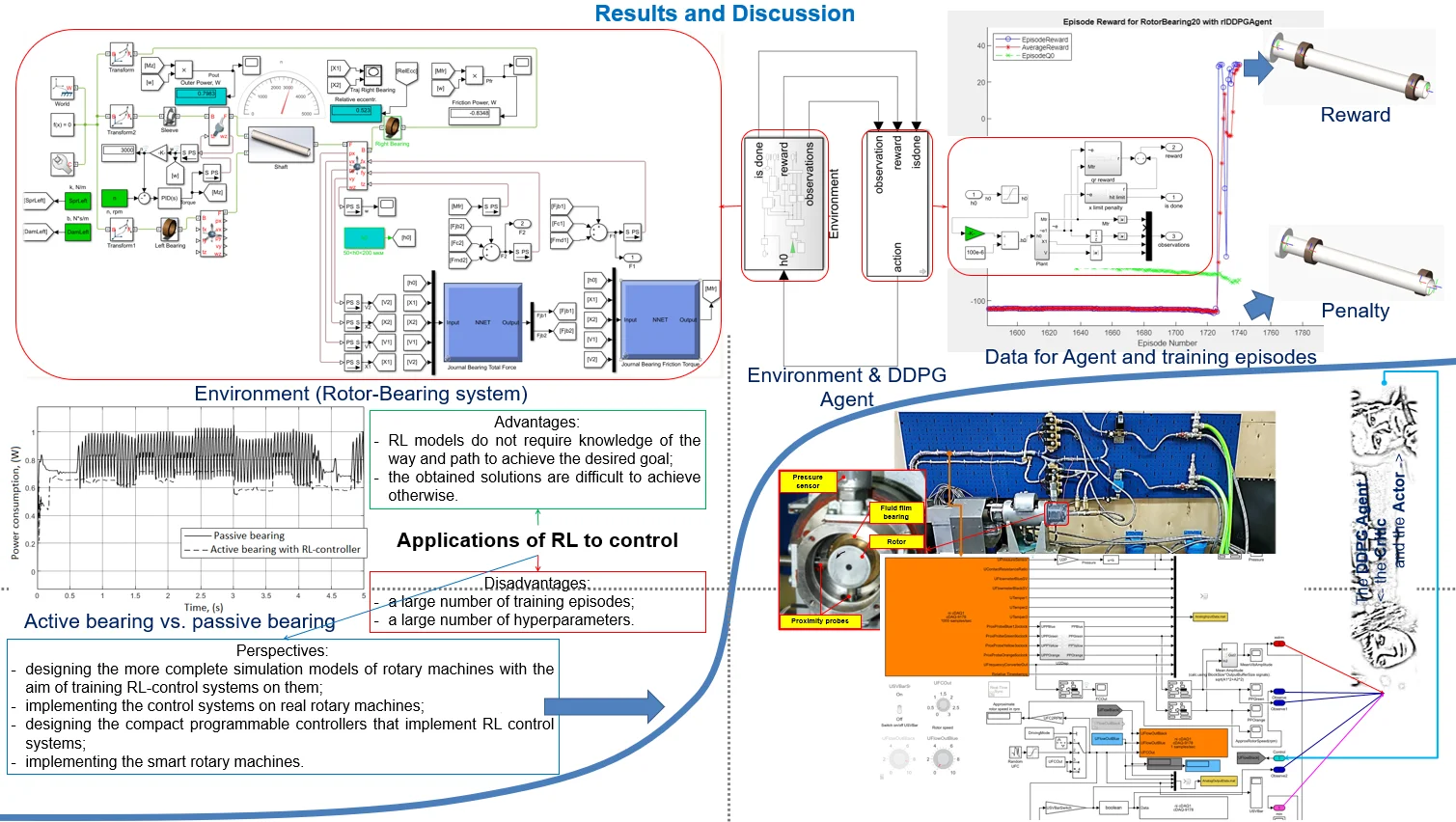
The main objective of the control system under study is minimization of energy consumption. The fluid-film reaction and the friction torque in a bearing are non-linear functions depending on pressure distribution (see Eq. (3)). It is assumed that the rotor vibrations described with Eq. (2), the coupling reaction $\mathbf{C}$ is linear and the bearing reaction $\mathbf{B}$ is simulated by the ANN described in Subsection 2.1 (see Fig. 2). In terms of reinforcement learning the rotor-bearing simulation model is an envinonment and the control system is an agent. At each time step $t$ the agent receives feedback from the environment ${\mathbf{S}}_t$ in form of a matrix of simulation results and takes an action $a_t$ in response in form of pressure supply or any other parameter of a fluid-film bearing. The main idea is to train agent after the event giving him higher reward $r_t$ for better actions.

The deep deterministic policy gradient (DDPG) is used. The algorithm of DDPG agents is represented in [8]. At each time step the value function $v_t$ is calculated as follows [8]:

where $\gamma$ is a discount factor, $q\text{'}$ is a $q$-function calculated by a target critic, $\mu \text{'}$ is a policy function of the action by a target agent, ${\mathbf{\Theta }}^{\mu }$, ${\mathbf{\Theta }}^q$ are unknown parameters of the actor and the critic ANNs respectively.

The architectures of the networks will be represented in the next section of the paper. The unknown parameters are calculated by minimizing the loss function [8]:

The networks are trained with stochastic gradient descent method using functions of specialized programming environments [9, 10].

4. Simulation and experimental results

The first series of simulation tests was performed with a model of the test rig based on Eqs. (2-4). A set of rotor trajectories was calculated. Then the ANN described by Eqs. (5-6) was trained and tested in comparison with a known linear model characterized by the spring and damper matrices [4]. The results demonstrated that the rotor dynamics simulation program with the ANN module allows calculation rotor trajectory two times faster than a real time process. It was demonstrated also that the ANN allows simulation of non-linear transient processes with variable rotor speed and high vibrations [4].

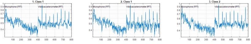
The second series of tests was performed using the test rig with a multi-sensor measurement system. Two displacement sensors measured the rotor vibrations, three vibroaccelerometers measured the rotor and the electromotor housings vibroaccelerations, a microphone measured the operating rotor machine noise. Inside the bearing the pressure sensor measured pressure supply and the contact resistance sensor measured the fluid-film thickness. Six conditions of the test rig were studied, including the normal condition, the conditions with loosened bolts and the rotor unbalance condition. The general classification problem for six classes recognition and the simplified classification problem for two classes recognition (normal or abnormal) were solved. Several random samples of two classes dataset with 800 data points each are shown in Fig. 3

Fig. 3Random samples of two classes dataset with normalized measurements results from the microphone and from one of the vibroaccelerometers

Then the ANN described by Eqs. (7-8) was trained and tested to solve the classification problems. The accuracy of the two classes and the six classes recognition were up to 80 % and 90 % respectively. It should be noted, that the accuracy of the two classes classification by experts was up to 70 %. The value of accuracy means that classification process was close to random.

The third series of the tests was simulation. The rotor dynamics simulation model became an environment observed and controlled by an agent. The agent model was based on the DDPG algorithm (see section 2.3). The ANNs architectures are shown in Fig. 4.

Fig. 4The DDPG networks architectures: a) the actor network and b) the critic network [2]

a)

b)

The agent controlled the bearing clearance size $h$ (see Eq. (3)) directly, and indirectly the pressure distribution and the reaction forces in the bearing. The goal of the control system was minimization of power loss due to friction and vibration in the bearing. The ANNs were trained and tested. The results demonstrated decreasing the power loss up to 17 % by the DDPG agent.

5. Conclusions

Suggested tools of rotor dynamics simulation, condition classification and control based on artificial neural networks allow development of predictive modeling systems, fault diagnosis and control of energy efficient operation to design intellectual rotating machines. All the developed systems can be combined in one device. The following study is connected with design of the device which will be able to combine multiple functions of predictive modeling, fault diagnosis and control in interaction with a rotating machine.