Fault diagnosis of rotating machinery under time-varying speed based on order tracking and deep learning

1. Introduction

As the mechanical equipment become larger and more complicated, it is more and more difficult to implement health condition monitoring and fault diagnosis. However, these large machines are often the core equipment in the production site, once the failure will cause serious economic losses and even safety accidents. Therefore, it is necessary to study appropriate fault diagnosis methods in real application scenarios. For rotating machinery, one of the most important reasons for poor diagnosis results is the fluctuation of rotation speed. Variations in speed, especially large speed variations, will lead to the failure of traditional time-domain and frequency-domain analysis, as well as difficulties in convergence of machine-learning-based fault diagnosis methods. So, it is necessary to realize intelligent fault identification by deep learning method after equal-angle sampling of signals by order tracking technology.

There has been a long time research on the variable speed analysis of rotating machinery. In the early research, computing order tracking (COT) is made mainly by arranging speed sensors to obtain speed signals [1]. On this basis of speed sampling, Vold-Kalman filter and other methods can be used to extract and analyze vibration signals of a specific order [2, 3], and equal-angle sampling method can be used to transform vibration signals from time domain to angle domain, so as to achieve order extraction of fault features [4]. However, the speed sensor cannot be installed in many tests, which makes the speed information difficult to obtain. TOT technique can be used for order extraction and rotation frequency fitting through time-frequency analysis, thus obtaining the virtual speed. But the TOT also has some shortcomings, especially the estimation is not accurate under large speed variations. Some scholars proposed improved methods of order tracking for this problem and achieved good results [5, 6]. After the equal-time sampling signal is converted into equal-angle sampling signal by order tracking, fault determination needs to be realized by means of fault feature extraction and identification. However, methods of fault diagnosis by vibration signal analysis are established on a large amount of professional knowledge. It is difficult to utilize the methods without sufficient knowledge of signal analysis. So, a large number of factories have a strong demand for intelligent diagnosis.

Deep learning is an effective feature identification method which can learn deep features to represent data distribution without prior knowledge and expert experience [7]. Deep neural networks (DNNs) can adaptively extract deeper and more essential features based on the internal structure of massive data than traditional machine learning model. DNNs have been successfully applied in many fields such as speech recognition, image classification, motion recognition, and text processing. In recent years, it has become an active trend to apply deep learning into fault diagnosis fault diagnosis research field. Xia et al. [8] designed a convolutional neural network (CNN) for fault detection and verified the method by Case Western Reserve University data and gearboxes data. Bruin et al. [9] used long short-term memory (LSTM) network for detection and identification of faults in railway track circuits. Furthermore, scholars have designed some novel deep learning models for fault diagnosis to solve variable-speed problems. Lu et al. [10] added a maximum mean discrepancy term to the loss function of auto-encoders to force them to learn features that are not affected by operating conditions. Qian et al. [11] proposed a new transfer learning method and solved data distribution problems caused by rotating speed variation. Peng et al. [12] proposed a novel deeper 1D CNN based on 1D residual block and the experimental results show that this method is effective in the case of strong noise and variable load.

Although in the above research, deep learning model shows many advantages. But the following problems are still not well solved.

1. There is a lack of research on the continuous variation of rotation speed. The existing data set usually has only a few data collected at a fixed speed. However, in reality, the variation of mechanical working conditions is usually continuous and uncertain.

2. Generally, the existing methods can only solve the problem of small range of velocity fluctuation, and lack of intelligent fault diagnosis methods under the condition of drastic and continuous changes of rotating speed.

Aiming at these problems, this paper combined with the advantages of order tracking technology and deep learning method, creatively proposed a rotating machinery fault diagnosis method based on TOT and long short-term memory and batch normalization (LSTMBN) to solve the intelligent diagnosis problem of time-varying rotating speed. Firstly, the TOT technology is used resample to the input signal to obtain the frequency domain periodic signal. Secondly, the frequency domain periodic signal is energy normalization using the RSN method. Thirdly, LSTMBN is used to extract temporal features and form a feature vector. Finally, the feature vector is fed into a fully connected (FC) layer and a softmax layer to obtain the fault classification category. The results of gearbox fault diagnosis experiment show that the model can effectively identify the faults and obtain higher fault diagnosis accuracy. The main contributions of this paper are summarized as follows:

1. A signal processing method under time-varying speed condition is proposed. Firstly, the angle-domain resampling of the signal is carried out by using the TOT technology, and then the influence caused by the speed change is eliminated by the RSN method.

2. A model based on LSTMBN intelligent diagnosis is proposed, which can improve the generalization ability of the model and enhance the robustness of the model.

3. A fault diagnosis method based on TOT and LSTMBN is proposed, which has higher accuracy and does not require domain knowledge and expert experience under the condition of varying rotating speed.

The remainder of the paper is organized as follows: In Section 2, the relevant knowledge is briefly described. In Section 3, procedure of the proposed method is illustrated. In Section 4, a gearbox fault diagnosis experiment is used to validate the effectiveness of the proposed method. Finally, conclusions are drawn in Section 5.

2. Relevant knowledge

2.3. LSTM model

In recent years, deep learning frameworks including auto-encoder (AE), deep belief network (DBN), CNN, recurrent neural network (RNN) and its variants [17, 18] has been developed for machine health monitoring. LSTM is an advanced RNN variant which can solve the problem of the disappearing gradient of the basic RNN [19, 20]. The forget gate in each time step unit enables LSTM to adaptively capture the long-term correlation and nonlinear dynamics of time series data [21]. Raw data as input is allowed in LSTM model [22, 23], and the literature [9] confirmed that LSTM is more suitable than CNN for fault diagnosis based on time series data.

Fig. 1LSTM cell structure

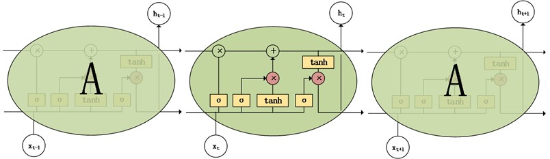
As shown in Fig. 1, the memory unit c is controlled through three gate structures in LSTM model. The input gate mainly controls inputting the temporary status information into the memory unit c; the forget gate mainly controls information which is forgotten at the last moment; the output gate is responsible for controlling whether the status information is output at this time. In the LSTM hidden layer unit structure diagram, $x_t$ is the input vector of the current sample, $h_{t-1}$ is the same hidden layer output, $h_t$ is the hidden layer output of the current sample, and the input gate includes two parts, $i_t$ and $a_t$. $f_t$ is the output of the forget gate, $o_t$ is the output of the output gate, $c_t$ is the update of the current state, and $c_{t-1}$ is the last state.

The LSTM single memory unit $c$ can be expressed as Eqs. (17-22):

17

$f_t=\sigma \left(W_f{h}_{t-1}+U_f{x}_t+b_f\right),$

18

$i_t=\sigma \left(W_i{h}_{t-1}+U_i{x}_t+b_i\right),$

19

$a_t=\mathrm{t}\mathrm{a}\mathrm{n}\mathrm{h}\left(W_a{h}_{t-1}+U_a{x}_t+b_a\right),$

20

$c_t=c_{t-1}°f_t+i_t°a_t,$

21

$o_t=\sigma \left(W_o{h}_{t-1}+U_o{x}_t+b_o\right),$

22

$h_t=o_t°\tanh \left(c_t\right).$

In Eqs. (17-22), $W$ and $U$ are weight matrices corresponding to each gate structure, and $b$ are biases.

3. Proposed method

The data-driven fault diagnosis method shows its advantages in condition monitoring. In recent studies, deep learning methods using multi-scale deep models have been able to realize fault identification under variable speed conditions. But these methods are based on the assumption that the rotating speed is fast and the machine does not need to start or stop frequently. It is impossible to realize effective fault identification in the stage of start-up and shutdown or the stage of large speed variation. At the same time, due to the limitation of field conditions, machines cannot be equipped with speed sensor, which makes the traditional order tracking method difficult to implement.

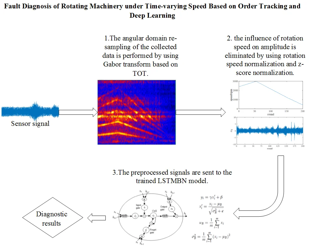
Accordingly, in order to solve the problem of intelligent fault diagnosis of time-varying speed, the intelligent diagnosis of equipment is realized by integrating TOT technology, speed normalization and LSTMBN model in this research. The framework of proposed fault diagnosis system for planetary gearbox is presented in the Fig. 2.

Fig. 2Flow chart of the proposed method

As it shown in the flowchart of preprocessing stage, firstly, the angular domain re-sampling of the data is performed by using Gabor transform based on TOT. After that, the influence of rotation speed on amplitude is eliminated by using rotation speed normalization and $z$-score normalization. The TOT based on Gabor transformation is shown in Fig. 3, and the details are described as follows.

Frequency spectrums of the collected signals are at first calculated by Gabor transformation. That’s because the Gabor transform is the best short-time Fourier transform and can well describe the instantaneous condition of signals with large changes. Afterwards, signal order extraction based on Gabor transform is carried out. In order to be suitable for large speed fluctuation and non-linear speed fluctuation, the center frequency is determined by linear interpolation of the order feature points in the Gabor time spectrum. This method can completely avoid the order recognition error caused by the interference of the spectrum ridges or the large fluctuations of the rotational speed caused by the interference. Then the Gabor coefficients of the corresponding order in the signal are obtained by the occlusion algorithm. The spectrum can be reconstructed by substituting Gabor coefficient into Eqs. (1-2), and the spectrum with only the $q$-th order component can be obtained. According to the local extremum search algorithm, the instantaneous frequency of the $q$-th order component is estimated, and the instantaneous frequency function is obtained. Further, the signals are re-sampled at the same angle by using the bond phase time scale method.

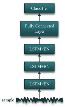
In the stage of training, a fault diagnosis method of LSTMBN model is proposed in this paper. The process is shown in Fig. 4, and the details are described as follows:

1) Data intercepting.

A sliding window is used to intercept the raw data to obtain samples $X\in R^L$, $L$ represents the length of the sample data sequence. It is clear that a small $L$ does not yield distinctive local features. On the contrary, if $L$ value is large, a large amount of global space-time information will be lost. Therefore, we select the appropriate length $L$ of sample data sequence through comparison experiments.

2) Feature extraction.

After obtaining sample $X$, LSTMBN model is used to extract the temporal sequence features of each component. The LSTMBN model is shown in Fig. 3. Two LSTMBN layers are used to extract the local temporal sequence features.

3) Batch normalization (BN).

The model parameters change constantly during the training process due to the multilayer structure. It leads to the continuous change of the input distribution of the subsequent layers. The learning process must adapt each layer to the new input distribution, so the learning speed must be reduced, which leads to the slower convergence rate of the model. Batch normalization layer normalizes the output of each layer into normal distribution, reduce the deviation of internal covariance and speed up the training process of deep model. The output calculation formula of BN layer is:

which, $x$ is the input vector, $x\in R^m$, ${\mu }_B$ is the mean value of $x_i$, ${\sigma }_B^2$ is the variance of $x_i$, $\epsilon$ is a very small constant, $\gamma$ and $\beta$ are the learned parameters in the model. BN can accelerate the convergence of the model and prevent overfitting. Using BN layer can reduce dropout rate and improve learning efficiency.

4) Defects classification.

Transfer the eigenvector v to another FC layer and classification layer. The formula is defined as:

which, $K$ is the number of labels, $\theta$ is a parameter of softmax layer.

Then calculate the error between the predicted value and the true value in the training data, the parameters of the whole model are trained by back propagation. Finally, the trained model can be applied to the machine health monitoring.

Fig. 3Flow chart of the proposed TOT method

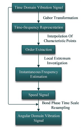
Fig. 4Flow chart of the proposed LSTMBN model

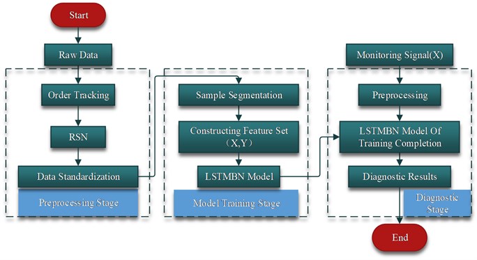
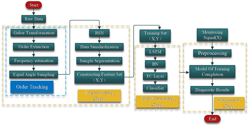
To sum up, detailed process of the fault diagnosis method proposed is shown in Fig. 5, and the details are described as follows:

1) For the collected signals$x\left(t\right)\text{,}$ the frequency spectrums are calculated by Gabor transformation.

2) An obvious order component is selected in the Gabor time-frequency diagram, and the filter center frequency line is obtained by connecting the control points placed on its ridge line.

3) The Gabor coefficient $C_{m,n}^q$ of the order is obtained by the masking algorithm, and the time spectrum $M_q(t,f)$ only for the order component is obtained.

4) Instantaneous frequency estimation and quadratic fitting is performed according to the local extremum search algorithm as in Eq. (9).

5) Bond phase time scale calculation and equal-angle re-sampling is performed by fitting the instantaneous frequency function.

6) Re-sampled signals are segmented.

7) Segmented signals constitute the $X\in R^{M\times T}$ of the sample sets $(X,Y)$. $M$ represents the number of samples; $T$ represents the length of data sequence.

8) The fault label $Y$ is added.

9) The sample sets are divided into training sets and test sets, and the appropriate batch size is selected.

10) Deep learning model is built.

11) The parameters of the deep learning model are selected.

12) The error between predicted values and truth values in training data can be calculated and back propagated to train the parameters of the whole model.

13) The monitoring signals are preprocessed.

14) The preprocessed signals are sent to the trained model.

15) Diagnostic results can be obtained.

Fig. 5The detailed flow chart of the proposed method

4. Experimental verification

4.1. Validation of speed estimation by simulated signal

Accurate speed estimation is the basis of high precision diagnosis. Therefore, we use the simulation signal of time-varying rotational speed vibration to verify the accuracy of the rotational speed estimation results of the order tracking method.

Taking the simulation signal of Eq. (28) as an example, the signal consists of three parts: impulse component, frequency conversion and harmonics caused by rotation, and noise:

28

$x\left(t\right)=\sum _{i=1}^{32}{A}_{i}s\left(t-T_i\right)+\sum _{n=1}^3{B}_n\mathrm{c}\mathrm{o}\mathrm{s}\left(2\pi nf\left(t\right)+{\beta }_n+N\left(t\right)\right).$

In Eq. (28), $A_i$ is the amplitude of the $i$-th impact, $T_i$ is the moment when the $i$-th impact occurs, the frequency at which the impact occurs is 1.75 times the rotational frequency, $B_n$ is the amplitude of the nth harmonic, and ${\beta }_n$ is the nth time. The initial phase of the harmonic, $s\left(t\right)$ is the impulse signal of Eq. (29), $f\left(t\right)$ is the instantaneous frequency shift of Eq. (30), and $N\left(t\right)$ is the noise:

29

${s\left(t\right)=e}^{-500t}\mathrm{s}\mathrm{i}\mathrm{n}\left(4000\pi t\right),$

30

$f\left(t\right)=\left[250+400\mathrm{c}\mathrm{o}\mathrm{s}\left(0.25\pi t\right)\right]/60.$

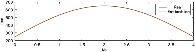
Take the time domain waveforms of the simulated signals of $B_1=$0.3, $B_2=$0.5, $B_3=$0.4, ${\beta }_1=\pi$/6, ${\beta }_2=-\pi$/3, $\beta \_3=\pi$/2 as shown in Fig. 6. The order tracking analysis of the simulated signal, the estimated speed and theoretical value obtained by the analysis are shown in Fig. 7.

It can be seen from the Fig. 7 that the speed estimation result is ideal, and the estimated value is not much different from the theoretical value.

Fig. 6Simulated vibration signal

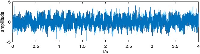
Fig. 7Revolving speed of the simulation signal

4.2. Comparisons of tests and results

4.2.1. Diagnostic object

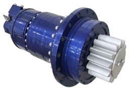
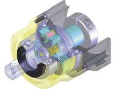
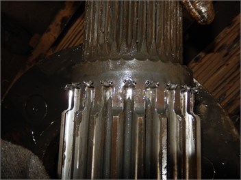
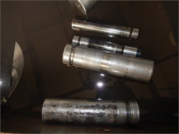
In the test, the turning gearbox with high workload and importance is selected as the diagnostic object. The transfer gearbox is a Siebenhaar CLP220 gearbox as shown in the Fig. 8(a), the gearbox is a three-stage gear, and its internal structure is shown in Fig. 8(b). Gear box failure types are tooth surface wear and bearing wear. Tooth surface wear is shown in the Fig. 9(a), bearing wear is shown in the Fig. 9(b). The method proposed in this paper uses the method of sample training to diagnose the fault, which can get rid of the expert knowledge and basic theory, so it does not need to know the internal structure of the gear box.

Fig. 8a) Siebenhaar CLP220 Slewing gear, b) internal structure of the gearbox

a)

b)

Fig. 9a) Defective parts of tooth, b) defective parts of bearing

4.2.2. Test method

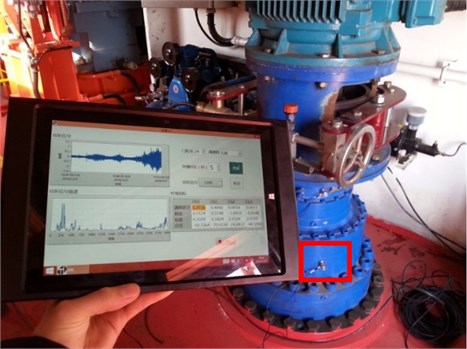
Due to the environmental constraints of the reduction gearbox, a portable data acquisition analyzer is used for vibration signal acquisition in the test. Gearbox is closed structure, the speed sensor cannot be placed on the test site. The field test is shown in the Fig. 10. The location of the accelerometer is shown in the red box in Fig. 10. The accelerometer is attached to the outside of the gearbox with a magnet, and the direction is parallel to the vibration direction.

In the experiment, LC0108T unidirectional piezoelectric accelerometer is used. Its parameters are shown in Table 1.

Table 1Parameters of LC0108T acceleration transducer

Sensitivity / (mV/g)	Range / g	Frequency Range / Hz	Mounting the resonance point / kHz	Resolution / g	Mounting thread /mm
500	10	0.35-4000	15	0.00004	M5

Fig. 10Field test

Because the door crane rotates manually by the driver, the working condition of the transfer gearbox is intermittent and non-uniform. In order to match the working condition, the starting and ending time of data acquisition is also controlled manually. The sampling rate is 10240 Hz. From October 16, 2015 to August 3, 2016, 14 turning gearboxes of 7 portal cranes were tracked and tested. 101 groups of valid samples were obtained through 20 tests. Among them, 18 # portal crane right-handed gearbox broke down in September 2015 and was repaired in October 2015.

4.2.3. Signal processing and sample allocation

The acquired vibration signal is preprocessed using TOT based on Gabor transform and RSN method, then the rotational speed is normalized by Eq. (23).

Fig. 11Vibration signal of left-handed rotation slewing gear

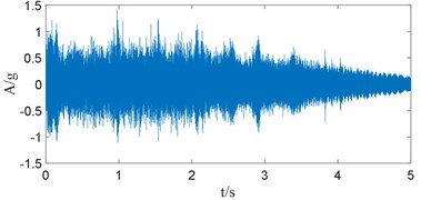
Fig. 12Resampled vibration signal

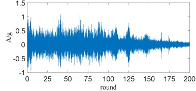
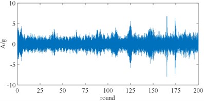
Taking the vibration data of a 15 # door reducer as an example, its time-domain waveform is shown in the Fig. 11. The signal sampled from equal angles is shown in the Fig. 12. Gabor time-frequency spectrum is shown in the Fig. 13. The speed curve fitted by order tracking analysis is shown in the Fig. 14. And the normalized signal is shown in the Fig. 15.

After re-sampling and normalizing vibration signals, the training sets and test sets are established. According to the known equipment failure situation, the training set and the test set are divided into two categories: fault and health. The input sample of the model is 1024 sub-signals, and the training sets and test sets are allocated according to the ratio of 0.25.

The Gabor time-frequency transformation is performed on the vibration signal shown in Fig. 11 to obtain the time-frequency map in Fig. 13. The trend of speed change can be clearly seen from Fig. 13; the local extreme value algorithm is used to extract the speed signal, and the data is resampled according to the speed signal to obtain Fig. 12. Fig. 14 is the estimated speed signal, by comparison with Fig. 13, it can be seen that the extracted speed signal can be consistent with the actual. It can be seen from the amplitude of Fig. 12 that the signal energy after resampling is still affected by the rotational speed, so the re-sampling data is normalized by the rotational speed, and the result is shown in Fig. 15. It can be seen from Fig. 15 that the vibration signal after pre-processing by the TOT and the RSN method substantially eliminates the influence of the rotational speed change on the signal.

Fig. 13Gabor time-frequency map of vibration signal of left-handed rotation slewing gear

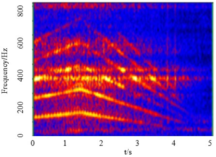
Fig. 14Rotating speed of left-handed rotation slewing gear

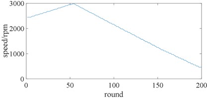
Fig. 15Normalized signal

4.2.4. Parameters of the LSTM

The architecture of the proposed method is built according procedures described in Section 3. It should be noted that the hyperparameters of the LSTM model are selected through cross-validated experiments. The hyperparameters such as cell number are displayed in Table 2. BN is used right after each main layer to improve the performance of the model. The activation function of the last layer is softmax and activation functions of other layers are all set to sigmoid.

Table 2Parameters of the LSTM model used in gearbox fault diagnosis experiments

No.	Layer type	Cell number	BN axis	Activation
1	LSTM	100	–	Sigmoid
2	LSTM	50	–1	Sigmoid
3	FC layer	10	–1	Sigmoid
4	Supervised learning layer	2	–	Softmax

The categorical cross-entropy is adopted as the loss function and Adam is employed for model training. The dropout rate is set to 0.2. Dataset is used to train the model for 20 epochs with the batch size of 10. The fault classification accuracy is used to evaluate the model performance.

4.2.5. Comparative experiments and results

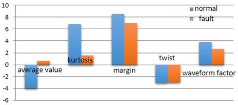
In this paper, the time-domain statistical indexes of vibration signals are compared with the proposed method. Time-domain statistical indexes are used to evaluate the vibration signal by five indicators: average value, kurtosis, margin, twist and waveform factor. The time domain statistical indexes of normal equipment and faulty equipment are analyzed, and the results are shown in Fig. 16. It can be seen from the comparison that the time domain indicator cannot effectively indicate the fault.

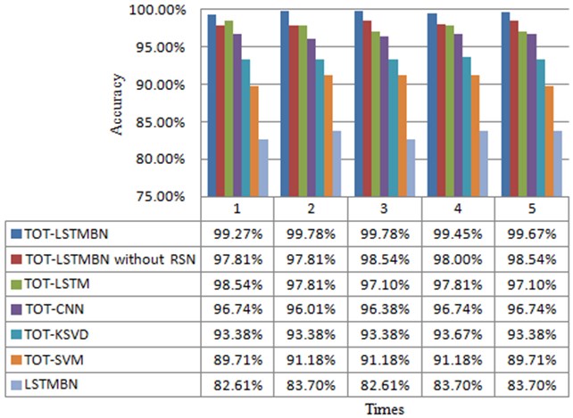
To prove the advantage of the proposed TOT-LSTMBN, the same sensor data is processed by some comparative models: the proposed network model (LSTMBN), TOT and feature-level fusion method based on support vector machine method (TOT-SVM), TOT and dictionary method (TOT-KSVD), TOT and convolutional neural network (TOT-CNN), the proposed TOT-LSTMBN model without batch normalization (TOT-LSTM) and the proposed TOT-LSTMBN model without RSN (TOT-LSTMBN without RSN).

In order to verify the essential role of TOT in time-varying speed, LSTMBN is adopted as a comparative model. The Parameter settings of the LSTMBN keep the same as the proposed TOT-LSTMBN model. To compare the performance of traditional fusion machine learning models based on handcrafted features with the deep learning models based on raw sensor data, TOT-SVM is adopted as a comparative model. In TOT-SVM, the data is decomposed by EMD firstly and the normalized energy, kurtosis, kurtosis and variance of the top five intrinsic mode functions are extracted as handcrafted features. All features are obtained to constitute a feature vector, which is used as the input of the SVM. To compare the performance of traditional machine learning models with the deep learning models based on raw sensor data, TOT-KSVD is adopted as a comparative model.

Fig. 16Result of time domain statistical analysis

It should be noted that, all the deep learning models in this experiment are consist of five main layers. The last two layers in each model are a FC layer with size of [100] with dropout and a softmax layer with size of [2]. In CNN, three pairs of convolutional layers and pooling layers are stacked. The filter size, stride and pooling size of three pairs of layers are set to [(4, 1), (4, 1), (2, 1)], [(1, 4), (1, 1), (2, 1)] and [(2, 1), (1, 1), (2, 1)] respectively. Parameters of the proposed TOT-LSTMBN are shown in Section 4.2.4. The Parameter settings of the TOT-LSTM keep the same as the proposed TOT-LSTMBN model, except that all the batch normalization layers are removed. The Parameter settings of the TOT-LSTM without RSN keep the same as the proposed TOT-LSTMBN model, except that the data are not normalized for rotational speed.

The testing results are listed in Fig. 17. It is shown that our proposed TOT-LSTMBN model can diagnose the faults of the gearbox effectively with the highest test accuracy.

As shown in Fig. 17, All models with order tracking are superior to those without order tracking, which is also expected, because order tracking converts non-stationary time-domain signals into stationary angular periodic signals, eliminating most of the influence of repetition on signal characteristics.

After order tracking, all the deep learning models based on raw sensor data can achieve better performance than the shallow machine learning model, which can be explained that the deep model can adaptively extract the deep sensitive fault features.

The proposed TOT-LSTMBN model can achieve higher test accuracy than TOT-CNN, which can be explained that the proposed TOT-LSTMBN model can extract temporal features of time series, which enables the TOT-LSTMBN layer to discover more hidden information than TOT-CNN.

The comparison of TOT-LSTMBN and TOT-LSTM proves that BN can improve the fault diagnose accuracy of the model. The comparison of TOT-LSTMBN and TOT-LSTMBN without RSN proves that RSN can improve the fault diagnose accuracy of the model. In the case of drastic rotation speed change, although the angular domain period is stable after re-sampling, the energy change caused by rotation speed still has an impact on the extraction of fault sensitive features. RSN normalizes the data according to the estimated rotational speed information eliminating the influence. Therefore, the proposed model can deliver better performance under the condition of drastic rotation speed change.

Fig. 17Comparative result

4.2.6. Feature visualization

As we know, deep learning models work like a black box, so it is hard to understand its process of extracting features. In this section, the t-SNE method is used to show the features extracted in our proposed model. T-SNE is an effective dimensionality reduction method, which can help us to visualize high-dimensional data by mapping the data from high-dimensional space to a two-dimensional space. Features extracted by each layer are respectively converted to a two-dimensional feature map. The feature maps of raw data and the FC layer are shown in Fig. 18, in which features of different types are distinguished by different colors. As shown in the Fig. 18(a), raw data of two types are all mix together; in the Fig. 18(b), until the FC layer, the features of the two types is separated and the features of the same type is clustered.

Fig. 18Feature visualization

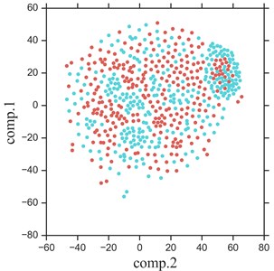
a) Raw data

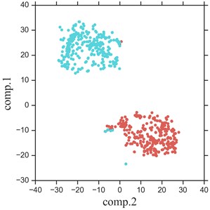
b) FC layer

5. Conclusions

In this paper, an intelligent fault diagnosis method based on TOT and LSTMBN was proposed. With the Gabor transform and the TOT combination algorithm, rotating speed can be estimated accurately without tachometer signal as reference. Based on this, the proposed method is capable of diagnosing faults under varying rotating speed. Furthermore, the RSN method is applied to solve the problem that the signal energy varies with the speed. The effectiveness was verified by detection fault on gearboxes and an accuracy of 99.78 % on fault detection approaches with varying rotating speed was achieved. It shows that the proposed method is potentially applicable for fault detection and location of planetary gearboxes in wind turbines. In the future research, the proposed method will be applied to other complex rotor-bearing systems, especially for diagnosis of distributed gear and bearing faults under more extensive non-stationary operating conditions.