Development of the theory of vibratory injection of gas into liquid

1. Introduction

The phenomenon of vibratory injection or vibroinjection was first recorded in 2000 by the joint laboratory of Mekhanobr-Tekhnika REC and the Institute of Problems of Mechanical Engineering of RAS [1] in the framework of research using the universal vibration stand [2]. The phenomenon may be illustrated as follows. Let us assume a system consisting of a vessel with water, performing vertical harmonic oscillations, and a small orifice in the bottom of the vessel. Under sufficiently intense oscillations of the vessel, air suction into the vessel is observed. Namely, within a single oscillation period, a gas bubble is formed and detached above the opening, and a liquid drop flows out the vessel. The theory of vibratory injection has been previously developed based on the key assumption that gas flows into the vessel when the pressure above the orifice is below the atmospheric pressure [3]. Namely, in the reference frame of the vessel, the pressure of the water column onto the vessel bottom is $p=p_0+{\rho }_l\left(g-A{\omega }^2\sin \omega t\right)h$, where $p_0$ is the atmospheric pressure, ${\rho }_l$ is the density of the liquid, $g$ is the acceleration of gravity, $h$ is the height of the liquid column, $A$ is the oscillation amplitude of the vessel, and $\omega$ is the oscillation frequency of the vessel. At the moments when $g-A{\omega }^2\sin \omega t<0$, gas enters the vessel; and when $g-A{\omega }^2\sin \omega t>0$, water flows out of the vessel. By developing this idea, simple formulas have been obtained, which may be used to predict the liquid and gas flow, as well as the size of the gas bubbles.

Additional experiments in a wider range of parameters ($A{\omega }^2<4g)$ indicate a deviation of the experimental data from the classical theory. Namely, it fails to predict the final gas bubble sizes, which result to be much smaller; and, therefore, it cannot predict the gas flow rate during vibratory injection. This suggests that the theory of this phenomenon has not yet been fully explained. The work presented covers further development of the theory of vibratory injection.

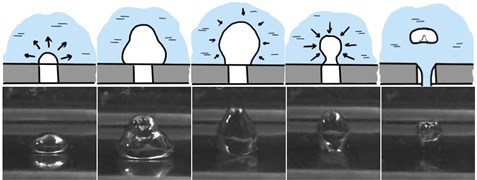
A series of experiments were carried out, with the measurement of gas and liquid flow rates, as well as high-speed video recording of the process. The use of an Evercam 4000-32-M high-speed camera enabled detailed monitoring of bubble formation (Fig. 1) and confirmed a more sophisticated physics of this process than previously used in the classical theory.

In this paper, we simulate the phenomenon of vibratory injection using the boundary integral method [4, 5] and discuss in more detail the physics of the process of gas vibratory injection into a liquid.

Fig. 1Bubble formation in vibratory injection. Bubble images were taken using an Evercam 4000-32-M high-speed camera

2. Basic equations

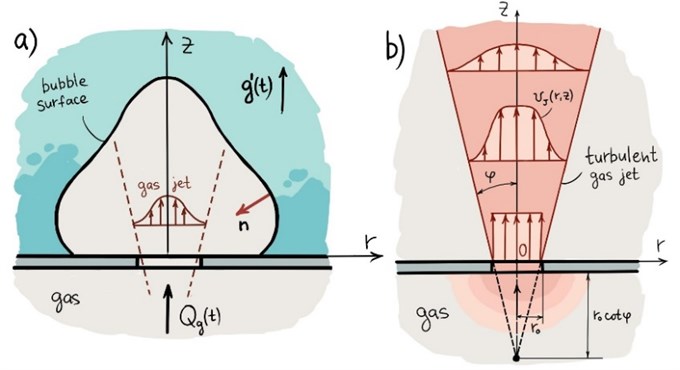
The liquid is assumed to be ideal and incompressible. Let us introduce a cylindrical coordinate system ($r$, $\alpha$, $z$) with the origin at the center of the orifice and direct the $z$ axis upward (Fig. 2(a)).

Assuming that the liquid motion is potential, let us introduce the velocity potential $\varphi$, to be defined using the liquid velocity as $\mathit{\upsilon }=\nabla \varphi$. Then, the continuity equation $\mathrm{d}\mathrm{i}\mathrm{v}\mathit{\upsilon }=0$ will be written in the terms of the potential as follows:

where $\nabla =\left(\frac{\partial }{\partial r},\frac{1}{r}\frac{\partial }{\partial \alpha },\frac{\partial }{\partial z}\right)$ is the nabla operator.

Fig. 2a) Schematic drawing of a bubble formed, b) structure of the turbulent gas jet inside a bubble

For the numerical solution of the problem, the Laplace equation of Eq. (1) may be conveniently rewritten as an integral equation using the Green theorem:

where $\mathit{r}$ is any point in the volume of the liquid or on its surface. If $\mathit{r}$ lies inside the liquid volume, then $c\left(\mathit{r}\right)=4\pi$; and if it appears on the surface of the liquid, then $c\left(\mathit{r}\right)=2\pi$; where $\mathit{r}\text{'}$ is any point on the surface of the liquid, and $G(\mathit{r},\mathit{r}\text{'})$ is the Green function. The p.v. designation implies that the integral is understood in terms of the principal value. The normal $\mathit{n}$ is oriented outward relative to the liquid volume under consideration.

In our problem, the liquid is limited by the bottom of the vessel, its side walls, the free surface of the liquid, and the surface of the bubble. At the bottom of the vessel $z=0$, the condition of ${\nu }_z=\partial \varphi ⁄\partial z=0$ must be true, meaning that the liquid cannot leak through the vessel bottom. Further, let us assume that the distance from the orifice to the side walls of the vessel and the free surface of the liquid significantly exceeds the orifice radius, and therefore the liquid occupies the half-space. In order to automatically satisfy the boundary condition of $\partial \varphi ⁄\partial z=0$ at $z=0$, it is convenient to introduce the images of all points of the bubble surface “below” the plane of $z=0$ and to solve the problem in the entire space, with the Green function taking the following form:

where $\stackrel{-}{\mathit{r}}\text{'}$ is the image of point $\mathit{r}\text{'}$ relative to the plane $z=0$, i.e. if $\mathit{r}\text{'}=\left(r,\alpha ,z\right)$, then $\stackrel{-}{\mathit{r}}\text{'}=\left(r,\alpha ,-z\right)$.

Let us break the bubble surface into $N-1$ parts in the form of horizontal conical rings. The contact lines of the rings (as well as the contact line with the vessel bottom) will be denoted as ($r_j$, $z_j$), where the $j$ index will take the values from 1 to $N$. Along these lines, all functions (potential, pressure, etc.) have the same value due to the axisymmetry of the problem. Given this discretization of the bubble surface, the integral equation of Eq. (2) will be converted into a linear algebraic equation of the following form:

This may be used to find the derivatives of ${\partial \varphi }_j/\partial n$ for the known ${\varphi }_j$. The matrices of $A_{ij}$ and $B_{ij}$ depend only on the bubble surface geometry and have the same form as in [6-8]. Using interpolation with cubic splines, the known ${\varphi }_j$ may be used to obtain the tangent derivative of the potential ${\partial \varphi }_j/\partial s$ along the bubble surface (the $s$ coordinate is measured along the bubble in the meridional direction). For the sake of simplicity, let us assume the boundary conditions for the cubic splines method in accordance with [6], namely:

The known ${\partial \varphi }_j/\partial n$ and ${\partial \varphi }_j/\partial s$ may be used to obtain the velocity of the points on the bubble surface.

Let us use the Bernoulli integral to establish the velocity potential value $\varphi$ on the bubble at each step as follows:

where $p$ is the liquid pressure on the surface of the bubble. Given the surface tension forces, it is related to the pressure in the bubble as $p=p_b+∆p-\sigma \kappa$, where $p_b$ is the gas pressure in the bubble, $\kappa$ is the local curvature of the bubble, $g\text{'}\left(t\right)=g(1-w\mathrm{s}\mathrm{i}\mathrm{n}\omega t)$ is the acceleration of gravity in the reference frame of the vessel, $w=A{\omega }^2/g$ is the overload parameter (assuming $w>$1), $A$ is the oscillation amplitude of the vessel, and $\omega$ is the oscillation frequency. Special attention should also be paid to the value of $∆p$, which is an additional contribution to the pressure due to the momentum of the gas entering the bubble [9]. Vibratory injection is only possible because of the high gas velocity when flowing into the bubble (otherwise, the bubble would be flattened along the bottom). The turbulent jet pressure of the inflowing gas will be calculated by the formula of $∆p=(1/2){\rho }_g{\upsilon }_{\mathrm{J}}^2\theta \left(Q_g\right)$, where ${\upsilon }_{\mathrm{J}}$ is the jet velocity and $\theta \left(x\right)$ is the Heaviside function, required to “disable” $∆p$ when the gas supply to the vessel stops. Let us assume that the jet velocity has a Gaussian profile [10], then:

Moreover, let us assume the jet angle of $2\phi \approx$ 24° (i.e. $\tan \phi \approx$ 1/5), see [10]). The jet structure is shown schematically in Fig. 2(b).

The gas flow through the orifice will be defined as:

where ${\rho }_b$ is the gas density inside the bubble and ${\rho }_g$ is the gas density outside the vessel, $\mu$ is the orifice coefficient. Assuming the approximation of ${\rho }_b\approx {\rho }_g$, the pressure in the bubble will be:

here, the sign($x$) function was added, which is +1 if the argument is positive, and –1 if it is negative. This is necessary in order to take into account any gas leakage from the vessel during bubble compression.

The Bernoulli integral may, therefore, be written as:

where $\mathrm{D}/\mathrm{D}t=\partial /\partial t+v\bullet \nabla$ is the material derivative.

The Lagrangian description will be used for the bubble surface. Namely, let us track the trajectories of the liquid particles that form the surface of the bubble. Their coordinates in the time interval of $\mathrm{\Delta }t$ will change as follows:

where the velocity projections of the points on the bubble surface are calculated using the derivatives of $\partial \varphi /\partial n$ and $\partial \varphi /\partial s$. The potential will have the increment of:

Due to the fact that we take into account the surface tension forces, the time interval $∆t$ must be less than the characteristic “capillary time” ${∆t}_{\sigma }=\sqrt{{\rho }_l{r}_0^3/\sigma }$ (see [11]).

The gas flow rate will be self-consistently determined according to the following formula:

the minus sign is due to the fact that the normal $n$ is directed inside the bubble, so the projection of the liquid velocity on the normal line to the bubble surface is ${\upsilon }_n=-\partial \varphi /\partial n$.

3. Initial conditions

Let us assume that, at the initial moment of time, the surface of the bubble is a hemisphere with the radius of $r_0$ and expands uniformly with the velocity of $U$. According to full-scale experiment data, the initial bubble injection time is $t_0\sim \pi /2\omega$. Let us take the initial velocity of the bubble surface as $U\sim (\mu /2)\sqrt{{\rho }_{l}gh(w-1)/{\rho }_g}$. The potential on a spherical bubble is $\varphi =-U{r}_0$.

4. Calculation algorithm

Using the known coordinates of the points of ($r_j$, $z_j$) forming a hemisphere at the initial moment of time $t_0$, the matrices of $A_{ij}$ and $B_{ij}$ are established. The known initial potential ${\varphi }_j$ is used to establish the normal derivatives of $\partial {\varphi }_j/\partial n$ by solving the equations system of Eq. (4); then, cubic splines are used to obtain the derivatives of $\partial {\varphi }_j/\partial s$. Using the potential derivatives obtained, the velocity of the bubble surface is established according to the formula of $\upsilon =\nabla \varphi$. The formulas of Eqs. (11-12) are used to establish the new points of ($r_j$, $z_j$), as well as new the potential on the bubble ${\varphi }_{j\mathrm{}}$ at the time $t_0+∆t$. The procedure is then repeated. The calculations render the shape of the bubble surface as it evolves, the time of detachment of the bubble from the vessel bottom, and the total bubble volume.

5. Calculation example

Let us assume the following parameters: the orifice radius of $r_0=$1 mm, the liquid column height of $H=$ 80 mm, the vessel oscillation frequency of $\nu =$ 30 Hz, the oscillation amplitude of $A=$1 mm, the orifice coefficient $\mu =$ 0.6, the liquid density of ${\rho }_l=$1000 kg/m³, the gas density of ${\rho }_g=$1.23 kg/m³, and the surface tension of $\sigma =$0.073 N/m. The calculation results are shown in Fig. 3. The curves are plotted via the points of ($r_j$, $z_j$) using cubic splines.

Fig. 3Bubble formation during vibratory injection: a) growth phase, b) collapse phase

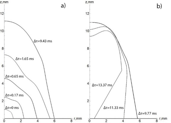
The bubble formation process took approximately $∆\tau \approx$0.013 s, which is comparable to the vessel oscillation half-cycle of $\pi /\omega =$0.016 s. The radius of the final bubble is approximately $r\sim$4 mm, which is observed in the experiment. Similar calculations may be performed with other parameter values.

It may be seen that, during its formation, the bubble has an approximately conical shape. Its vertical elongation is due to the momentum of the high-velocity jet of gas flowing into the vessel; and the horizontal elongation of the bubble near the bottom of the vessel is caused by the reduced hydrostatic pressure at this point (since $g^{\text{'}}<0$, and the hydrostatic pressure rises in the direction of the axis of $z$). When the acceleration direction of the vessel changes its sign, the pressure in the liquid rises, and the bubble contracts, reducing its size as the gas flows out of the vessel during compression. Since the pressure increase is higher near the bottom of the vessel and the liquid at the top of the bubble cannot instantly change its motion direction due to inertia, the bubble begins to collapse from below (at the bottom of the vessel), thereby forming a neck region, which hinders gas leakage, simultaneously leading to bubble detachment from the vessel bottom.

6. Conclusions

On the basis of detailed experimental data on the formation of gas bubbles during vibratory injection, a more comprehensive explanation from the point of view of physics for the phenomenon has been provided. A theory describing gas vibratory injection into liquid at the acceleration parameter not exceeding 4g has been suggested.

An important factor in bubble formation is the presence of a high-velocity jet of gas, which accelerates the liquid near the orifice and gives the bubble an elongated vertical shape. The bubble formation proceeds in two stages namely bubble growth upon gas injection into the vessel and the subsequent collapse of the bubble with the outflow of gas from the vessel. Due to the second stage, the bubble size tends to be smaller than expected.

Vibroinjection modeling using the boundary integral method allows predicting the final bubble size and the actual gas flow for vibroinjection. The results of numerical simulations are in good agreement with the experiment. The results of this study may be used in the design of gas dispersers based on the vibratory injection phenomenon.