An approach to fault diagnosis for gearbox based on order tracking and extreme learning machine

2.1. Computed order tracking

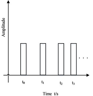
A method, obtaining the signal in the angular domain based on COT, depends on the rotational speed pulse (see Fig. 2). Compared with the hard order tracking, installing complex devices, COT can obtained rotational speed to install a tachometer to obtain resample signals. After resampling, the signal in angular domain, carried on the Fourier transform, then obtains the order domain. Sampling rate $O_S$ should meet the conditions of Eq. (1) because of the Nyquist sampling theorem:

where $O_{max}$, the maximum analysis order. And in order to ensure a full period sampling, the sampling number of each cycle should be $2^n$, $n$ equals 1, 2, 3….

Fig. 1The flow chart of the article

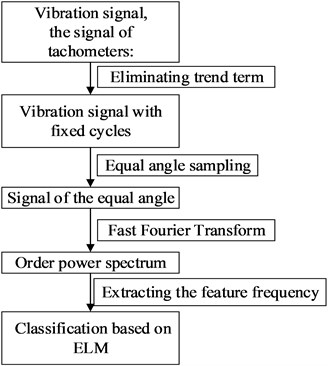
Fig. 2Rotational speed pulse signal

Angular resampling is the most important step in the realization of order tracking.

The steps of order tracking methods analysis [9]:

1) Function $n\left(t\right)$ fitted by keyphasor signal.

2) Calculating the angle function $\theta \left(t\right)=\frac{\pi }{30}{\int }_0^{t}n\left(t\right)$ of the reference axis.

3) Calculating the resampling time $t_n$, through the quadratic curve fitting. It is assumed that the shaft is undergoing constant angular acceleration. With this basis, the shaft angle, $\theta$, can be described by a quadratic equation of the following form:

The unknown coefficients $b_0$, $b_1$, $b_2$ are found by fitting three successive keyphasor arrival times $(t_1,t_2,t_3$), which occur at known shaft angle increments $\mathrm{\Delta }\varphi =2\pi$

Then, this yields the three following conditions, $\theta \left(t_1\right)=0$; $\theta \left(t_2\right)=\mathrm{\Delta }\varphi$; $\theta \left(t_3\right)=2\mathrm{\Delta }\varphi$:

In the formula, $t_n$ is the time when the angle of ${\theta }_k$ is turned around.

4) Calculating the vibration data $x^{\mathrm{\text{'}}}\left(\mathrm{}{t}_n\right)$ of the equivalent angle by interpolation of the original vibration signal $x\left(\mathrm{}{t}_n\right)$, and interpolating functions are as follows:

In the formulas, $t_s$ denotes the interval of sampling in the time domain, the value of $k$ makes that $k{t}_s$ and $t_n$ are the closest, $h_s$ is the interpolation filter, $h_s\left(t\right)$ is the interpolation function.

2.2. Extreme learning machine

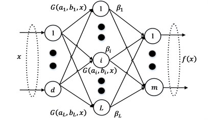
Single-hidden layer feedforward neural networks (SLFNs) algorithm, the structure shown in Fig. 3, is the basis of ELM. Compared with the traditional SLFNs algorithm, ELM is a novel algorithm of SLFN, which has lots of advantages. Obviously, ELM could randomly produce weight between hidden layer and input layer and the thresholds of hidden layer nodes are also stochastically. Furthermore, while training the network, ELM can avoid to adjust weights or thresholds. Simply speaking, the algorithm only needs to set the number of hidden layer neurons to get the unique optimal solution. And learning pace of ELM is very quick and it shows good generalization performance. As follow, the Eq. (7) is the mathematical model of ELM [12, 13]:

In the Eq. (7), $g_i$ expresses the output function $G_i\left(a_i,\mathrm{}{b}_i,\mathrm{}x\right)$ of the $i$th node which belongs to the hidden layer.

Fig. 3Single-hidden layer feedforward network

For a neural network, the activation function is very important. For ELM, the activation functions of the hidden layer usually have three types:

In [12, 13], the authors made a statement of advantages and explain that three types of activation functions show good performance. And in this paper, Eq. (8) is selected as the activation function. The steps of ELM algorithm as follows:

1) Determine the number $L$ of neurons in the hidden layer and activation function $g\left(x\right)$, and randomly assign $a_i$, $b_i$, ${\beta }_i$.

2) Calculate the output vector of $i$th.

3) Calculate the output weight $\widehat{\beta }$.

3.1. Experimental facilities

The source of the data in this paper comes from the 2009 PHM Conference Data Analysis Competition. The data is about gearbox made of 560 samples which are constituted two types of gearboxes and fourteen kinds of fault modes. And each of the working conditions has different shaft speeds 30, 35, 40, 45, and 50 Hz and four kinds of loads. And the author chooses four typical fault modes (see Table 1) to verify the feasibility of the new algorithm proposed [4].

3.2. Order tracking and feature extraction

1) Data resampling. In order to reduce system error of the signal, which could be caused by the sensor, signal preprocessing of eliminating trend was implemented. Then COT was used to transform the non-stationary vibration signal of time domain into the stationary signal of angular domain, this paper uses a method named computed order tracking.

Autocorrelation Coefficient (ACF) [14] is calculated to compare the stability of signals both time domain and angular domain. Autocorrelation Function, effective method to inspect the stability of time series while vibration signal is a kind of time series.

From the Fig. 4, the details of ACFs presented, we can see that the convergence rate of the ACF of signal in the angular domain are faster than the other, which verify the angular signal is more stable than the time signal.

2) Characteristic Parameters Extraction. In this section, characteristic vector was extracted. First, Fast Fourier transform is applied to the angular resampling signal, thus the order power spectrum can be obtained (see Fig. 5). There was six feature order selected as follows: $W_1$ represents the order power spectrum of order 32; $W_2$ represents the order power spectrum of order 64; $W_3$ represents the order power spectrum of order 96; $W_4$ represents the order power spectrum (PS) of order 128; $W_5$ represents the order power spectrum of order 48; $W_6$ represents the order power spectrum of order 80. Then the characteristic parameters of each characteristic order are $W_j$, $j$ equals 1, 2, 3, 4, 5, 6.

Because of different energy distributions under different operating conditions, it is feasible to use the energy percentage of feature orders as the feature vector. Then the feature parameters are normalized:

$w$, sum of the characteristic parameters $W_j$, that means $W=\sum _1^6{W}_j$, $j$ equals 1, 2, 3, 4, 5, 6. ${\overline{W}}_j$, the normalized parameters of $W_j$. $T$, the feature vector after normalization processing.

Fig. 4The ACFs of different fault modes

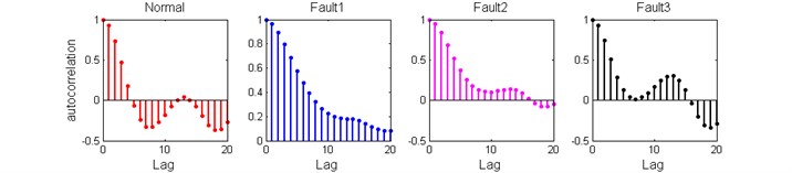
a) ACFs in the time domain

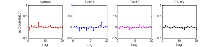
b) ACFs in the angular domain

Fig. 5Order power spectrum under different conditions

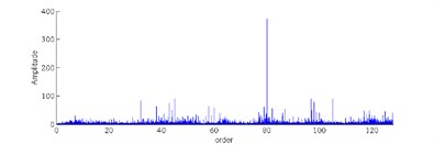
a) Normal

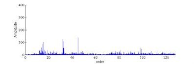
b) Fault 1

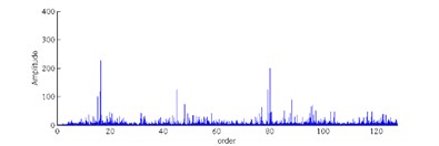
c) Fault 2

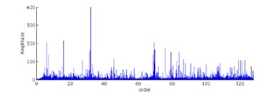
d) Fault 3

3) Fault diagnosis based on ELM.

There are 60 samples in each case. 50 samples are used as training samples for the ELM and the rest samples are used as testing samples for the ELM. By the way of cross validation, the classification performance is showed. The final classification accuracy is the average of the results of the 300 ELM’s classification (see Table 2).

Based on the COT-PS-ELM approach, the fault detection results under different loads are studied. The result of fault diagnosis shows on Table 2. From the Table 2, the COT-PS-ELM method shows the accuracies of total are 0.9908, 0.9803, 0.9147, 0.9420 and all of them are greater than 90 %. It is also found that the accuracies of low loads are higher than high loads. Thus, it can be seen COT-PS-ELM is more suitable for low load conditions.