Abstract
This paper numerically computed the problem of pressure fluctuations in the open air and tunnel based on the virtual computer technology, and experimentally verified the correctness of the numerically computational model. In the open air, pressure fluctuation at the nose tip of train head was serious and presented two obvious valley and peak values. Pressure at the nose tip of train tail did not present obvious fluctuations. Pressure at the train head was obviously more than that at the train tail. For different observation points, the peak and valley values of far-field pressures only showed translation with the increased running time. In the tunnel, pressures at the nose tip of train head had obvious peak and valley values and were far more than those in the open air. For different observation points, the peak and valley values of far-field pressures did not simply present translation with the increased running time, which indicated that there was wall effect in the tunnel. In addition, the absolute values of the maximum positive and negative pressures of the high-speed train in the near and far fields obviously increased with the increased running time. The pressure fluctuation caused by the high-speed train in the tunnel was the superposition of the inlet pressure wave and air disturbance caused by the passing train. The size of local air pressure was related to tunnel length, train length and speed. The peak value of positive pressures in the tunnel appeared when the train entered the tunnel. The valley value of negative pressures in the tunnel would appear in the area where the expansion wave of train head was superimposed with the compression wave of train tail. According to tunnel length, train length and speed, the specific positions where the peak and valley values of positive and negative pressures appeared could be approximately obtained. If the tunnel was very long, it was possible to present the peak value of positive pressures caused by the superposition of more continuous compression waves or the valley value of negative pressures caused by the superposition of more continuous expansion waves.
1. Introduction
When a high-speed train enters a tunnel suddenly from the open air, space around the train will be small and air pressure will rise. In the meanwhile, a compression wave is caused at the tunnel inlet and spreads to the tunnel outlet at the speed of sound. When train tail enters the tunnel, the space occupied by the train body at the tunnel is suddenly released and air squeezed by the train body at the tunnel inlet is released, which suddenly reduces pressure and forms an expansion wave. The expansion wave will pass through the train and spread to the tunnel outlet at the speed of sound. The compression wave will convert to an expansion wave at the tunnel outlet and then spread to the tunnel inlet. If the tunnel is very long, the train will still run in the tunnel at this time. The expansion wave will also convert to a compression wave at the tunnel outlet and return to the tunnel inlet. Therefore, the pressure transient caused by the passing trains in a tunnel will discomfort drivers and passengers occasionally. In the development process of high-speed trains, tunnel pressure wave is an important aerodynamic problem. Studied results can provide an important reference for the design of tunnels and trains[1, 2].
At present, tunnel pressure wave is mostly studied by experiments. Meanwhile, a lot of achievements have been obtained. Yoon [3] studied the aerodynamic effect of a tunnel, conducted real train tests and analyzed the formation and propagation process of compression wave in the tunnel and the change rule of micro-pressure waves at the tunnel inlet. Suzuki [4] combined the experimental test with numerical simulation, and found that the aerodynamic pressures in a tunnel were an important factor for the strong vibration of the train. Fukuda [5] took advantage of real train measurement and one-dimensional numerical analysis, and conducted an aerodynamic analysis on a tunnel with a length of 26 km. Luo [6] adopted an aerodynamic model to study the propagation mechanism of transient pressure of a high-speed train in the process of entering a tunnel with buffer structure. Experimental results showed that the buffer structure could reduce transient pressure in the tunnel. Liu [7] adopted a real train to test the aerodynamic pressure of tunnel wall caused by the passing high-speed train through a double-track tunnel, and analyzed the peak values of pressures in different positions when the train passed through the tunnel. Zhang [8] measured the pressure of tunnel wall when a high-speed train passed through a tunnel, which was very important to study the aerodynamic performance of the high-speed train in the tunnel. However, there was a very high demand for the experimental environment and system. In the meanwhile, it was difficult to separate the problems of pressure fluctuation caused by mechanical vibration and air transmission.
In recent years, a number of scholars have conducted numerical computation for the high-speed train passing through a tunnel with the development of computational fluid mechanics [9-14]. Based on one-dimensional compressible unsteady flow model and generalized Riemann variable method, Jia [15] conducted a numerical simulation for a single train passing through a tunnel and two trains meeting in a tunnel, and studied the influence of train speed and blockage ratio on the maximum pressure and minimum pressure values outside the train. Based on one-dimensional compressible unsteady flow model and the parameter characteristics of tunnel section, Mei [16] studied the characteristics of pressure fluctuation of a single train passing through a super-long tunnel with simple structure, and concluded the influence of tunnel length, train speed and air tight index on pressure in the train. Bell [17] established a numerically computational model for a two-dimensional high-speed train passing through a wind tunnel, considered coupling effect and pointed it out that tunnel wall effect was the main reason for the formation of pressure waves in the tunnel. However, the mentioned numerical simulation was mainly aimed at one-dimensional and two-dimensional models and the detailed features of three-dimensional models were neglected. Based on CFD software, Xu [18] adopted the pressure correction algorithm of three-dimensional compressible unsteady turbulent flow models and the grid technology of arbitrary sliding interfaces to conduct a numerical simulation for the pressure waves of the high-speed train which met in a tunnel at a constant speed and a non-constant speed, respectively. However, computational results were not verified by related experiments. Li [19] conducted a simulation analysis on the process of a high-speed train passing through a tunnel through the three-dimensional numerical computation. Computational results proved the superposition relationship of pressure effect at the inlet and disturbance effect of the train passing through the tunnel. However, the pressure wave in the tunnel was not compared with that in the open air.
This paper numerically computed the problem of pressure fluctuations in the open air and tunnel, reflected the existence of tunnel wall effect through a comparative analysis, and experimentally verified the correctness of numerically computational model. The specific positions of the peak value of positive pressures and the valley value of negative pressures could be obtained through analyzing the pressure fluctuations in the tunnel under different speeds.
2. Numerical computation of pressure waves in the open air
2.1. Computational model and boundary conditions
A high-speed train was taken as the studied object. To reduce the computational work of CFD, a 2-train formation including a head train and a tail train was established, as shown in Fig. 1. The complete length of the train is 53 m, and the height of the nose tip is 1.2 m. To improve the computational precision, the turbulence model of compressible three-dimensional transient Reynolds time-averaged equation and RNG equation was applied to obtain aerodynamic forces. The physical model of the train in the open air was shown in Fig. 2.
Fig. 1Geometric model of the high-speed train
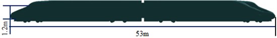
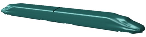
Fig. 2Computational model of the high speed train in the open air
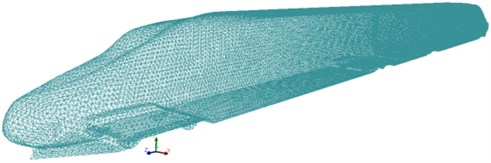
a) Grid model of the high-speed train

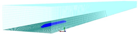
b) Front view of the computational domain
c) Three-dimensional view of the computational domain
The computational domain of external flow field is 500 m; interval under the train is 0.2 m; the computational domain of fluid was 60 m high and 90 m wide. The flow field was divided into dynamic grids and the fixed grids. The part of dynamic grids contained the area around the train. This area mainly paid attention to the translation of the train. Therefore, the method of dynamic grids was adopted. Grids around the train would not change in the process of computation. Grids which changed were mainly at two end faces in the part of dynamic grids. When the size of grids was more than the scheduled size of grids, grids would be split. Otherwise, grids would be combined. The part of dynamic grids slipped at the running speed of the train. The data transfer between dynamic grids and fixed grids was completed through establishing an interface. The model in this paper adopted tetrahedral grids. The number of boundary layers on the train wall was 8. The thickness of grids in the first boundary layer was 2.5 mm. The total number of grids in the model was 6,800,000. Boundary conditions were set as follows: Wall boundary conditions were adopted for the wall of the train and ground. As RNG equation was adopted, it was a model with a high Reynolds number. For the flow in the area close to the wall, Reynolds number was low. Therefore, wall function method was applied in the area close to the wall. Other external fields applied pressure far fields. Standard atmospheric pressure was 101 kPa.
2.2. Pressure waves in near field
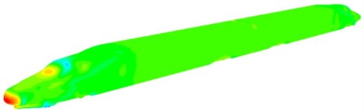
Based on the model and boundary conditions, pressures at the nose tip of train head and tail were numerically computed, as shown in Fig. 3. In addition, the contour for the pressure of train surface at a certain moment was extracted, as shown in Fig. 4. As displayed from Fig. 3(a), pressure fluctuations at the nose tip of train head were serious and showed two obvious valley and peak values in the running process. When running time was 2.6 s and 5.7 s, the valley pressures of the high-speed train were 2542 Pa and 2560 Pa respectively. When running time was 0.2 s and 4.8 s, the peak pressures of the high-speed train were 2667 Pa and 2645 Pa respectively. The difference value between the maximum pressure and the minimum pressure was 125 Pa. As displayed from Fig. 3(b), pressure at the nose tip of train tail showed no obvious fluctuations. When running time was less than 1.2 s, pressure dramatically decreased with the increased running time. However, pressure tended to be a stationary value when running time was more than 1.2 s. Additionally, pressure at the train head was obviously more than that at the train tail. This rule was also reflected by the distribution of contour for pressure in Fig. 4. Airflow firstly acted on the train head and extended to the tail along the train body. However, flow velocity would decrease and pressure would be reduced.
Fig. 3Pressures at the nose tip of train head and tail
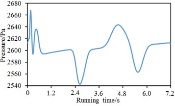
a) Nose tip of train head
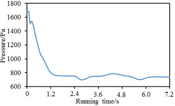
b) Nose tip of train tail
Fig. 4Pressure distribution on the surface of the high-speed train
2.3. Pressure waves in far field
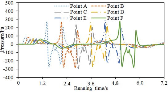
To compare with the subsequent pressure waves of the high-speed train in the tunnel, a virtual tunnel with a length of 250 m was set. 6 observation points were arranged horizontally and evenly. The distance between two adjacent observation points was 50 m. Observation points were 1 m away from the ground. The pressure waves of 6 observation points were extracted, as shown in Fig. 5. It could be seen from Fig. 5 that the pressure waves of 6 observation points showed similar changes. Translation only happened to peak and valley frequency points. In the open air, the pressure waves of 6 observation points were mainly from the compression wave brought by the motion of the high-speed train. For the observation point A, the first peak value was the pressure fluctuation caused by the train head which just passed through this position. For the other observation points, the situation was similar.
Fig. 5Comparison of pressure waves of 6 observation points
3. Numerical computation of pressure waves in the tunnel
3.1. Computational model and boundary conditions
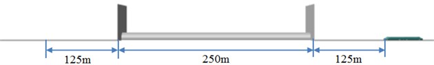
To simplify the work of grid generation, the three-dimensional numerical simulation of a single high-speed train entering the tunnel appropriately simplified the tunnel according to requirements, which formed a smooth pipe without various buildings in the tunnel and the topographical environment outside the tunnel and the thickness of tunnel. Due to the limitation of computational scale and time, the model computed the tunnel with a length of 250 m. The tunnel section had to satisfy the design requirements of high-speed railways, space outside the tunnel entrance and exit was 125 m long, whose width and height were more than 10 times that of train width, as shown in Fig. 6. To simplify computation, the following hypothesis was made for the model.
Fig. 6Geometric model of the high-speed train passing through the tunnel
Before the generation of grids, the first step was to determine the size of computational domain. The computational domain of model used in this paper contained train model, tunnel model and numerical computation space including limited external open space involved in the running process of the train in the tunnel. It was composed of three space regions including open space outside the tunnel, tunnel space and additional grid space. The shape of train was basically the same with the external dimension of high-speed trains. The structure of train connection was considered. However, the lower part of train body was simplified to a certain degree. The train only considered wheels and neglected the detailed structure of bogies and the outer surface structure of train body, such as windshield wiper, head light and door knob. The tunnel was plat and straight; the track was not sloped; the route was not curved. Tunnel and track walls were replaced by a hook face or a plane with certain surface roughness. When the train entered the tunnel at a high speed, air in the tunnel would be greatly compressed and considered as compressible fluid in the case of computation. When the high-speed train ran, external flow field was a steady flow field and RNG equation was adopted to simulate the steady state flow in the case of computation. Computation applied mobile grid technology to simulate the motion of the train. Namely, train and flow field around the train moved at a specified speed and grids of other flow fields kept still. Finally, the model of high-speed train passing through the tunnel was shown in Fig. 7. The total number of grids of the model was 17,000,000.
Fig. 7Computational model for the high-speed train passing through the tunnel

a) The whole model
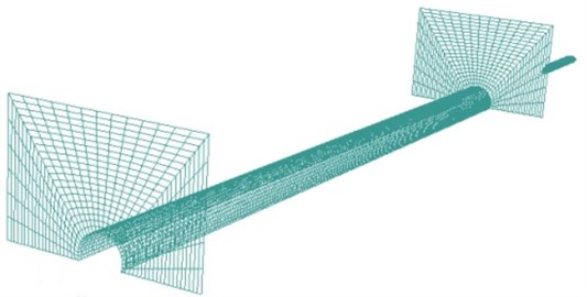
b) Local model of the tunnel
3.2. Pressure waves in near-field and far-field at the speed of 250 km/h
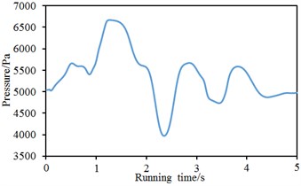
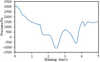
To compare with the pressure fluctuations of the high-speed train in the open air, the high-speed train still ran at the speed of 250 km/h in the tunnel and observation points were in the same positions. Based on computational model and boundary conditions, pressure waves at the nose tip of train head and tail were computed, as shown in Fig. 8. As displayed from Fig. 8, pressure fluctuations at the nose tip of train head were severe and showed two obvious valley and peak values at the running process of the high-speed train. When running time was 2.9 s and 4.4 s, the valley pressures of the high-speed train were 2167 Pa and 2280 Pa respectively. When running time was 2.1 s and 3.6 s, the peak pressures of the high-speed train were 3478 Pa and 3125 Pa respectively. The difference value between the maximum pressure and the minimum pressure was 1311 Pa. As displayed from Fig. 8(b), pressure drastically decreased with the increase of running time when running time was less than 2.1 s. However, pressure showed to obvious valley values, namely –350 Pa and –500 Pa after running time was more than 2.1 s.
Fig. 8Pressures at the nose tip of train head and tail
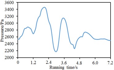
a) Nose tip of train head
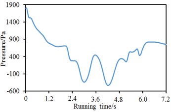
b) Nose tip of train tail
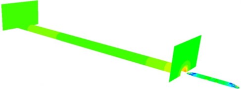
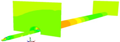
To verify the correctness of computational model for the high-speed train passing through the tunnel, the experimental test system was composed of a pressure sensor, IMC data acquisition system, wireless long-distance control system, wireless long-distance data transmission system and notebook computer. According to the requirements of experimental test specification, the experiment selected 1 kHz as sampling frequency. Filter frequency was 250 Hz. In the whole process of the experimental train passing through the tunnel, the deviation of train speed was controlled within 1 %. To exert no influence on the flow field of surface pressure around observation points, the experiment adopted a pressure-resistance sensor with the measurement range of 6.90 kPa, as shown in Fig. 9. The pressure sensor was calibrated before experimental test. Tested error was less than 1 %. Multiple dynamic pressure sensors were arranged at the nose tip of train head and tail. A comparison between experimental and numerical computational results was made, as shown in Fig. 10. As displayed from Fig. 10, numerical computational and experimental results showed good consistency at the nose tip of train head and tail, which indicated that the numerical model established in this paper was correct. The contours for the pressures of the high-speed train at different moments in the process of passing through the tunnel were extracted, as shown in Fig. 11. Fig. 11(a) showed the contour for the pressure of the high-speed train which did not enter the tunnel. At this time, the pressure of the high-speed train was not affected by tunnel wall effect and contours for pressures in the front and rear of train surface were basically the same. Fig. 11(b) showed the contour for the pressure of high-speed train which just entered the tunnel. At this time, the tunnel surface produced large pressure due to the interaction between compression and expansion waves. Fig. 11(c) displayed the contour for the pressure of the high-speed train which ran in the middle of the tunnel. At this time, pressures of tunnel surface were symmetrically distributed. Meanwhile, pressures at the train head and tail were relatively larger, which resulted from the interaction between compression and expansion waves. Fig. 11(d) displayed the contour for the pressure of the high-speed train which pulled out of the tunnel for some distance. At this time, the train pulled out of the tunnel. However, tunnel surface still showed very serious pressure fluctuation due to the existence of compression and expansion waves.
Fig. 9Experimental test on the pressure of the nose tip
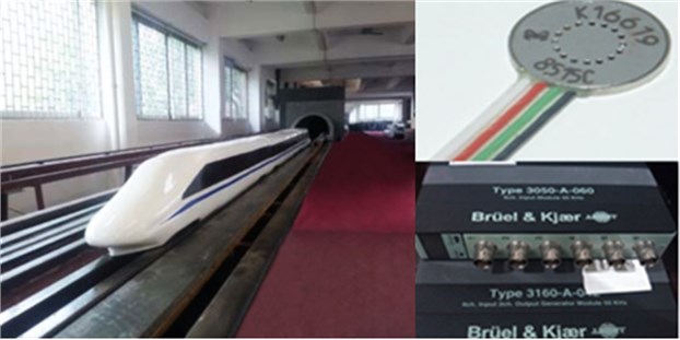
Fig. 10A comparison of experimental and numerical computational results
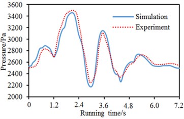
a) Nose tip of train head
b) Nose tip of train tail
Fig. 11Contours for the pressures of the high-speed train passing through the tunnel

a) 0.2 s

b)2.54 s

c)4.3 s

d)7.0 s
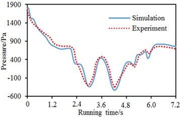
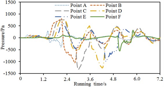
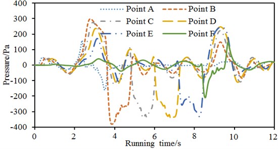
Pressure fluctuations of 6 observation points on the tunnel wall were extracted, as shown in Fig. 12. Through comparing it with Fig. 5, it could be seen that pressure fluctuation on tunnel wall was obviously different from that in the open air. In addition, pressure in the tunnel was more than that in the open air. It was because of the impact of tunnel wall effect. Observation point A and F were at the tunnel entrance and exit. Tunnel entrance was only affected by compression wave while tunnel exit was only affected by expansion wave. Therefore, two observation points were different from other observation points. To observe the impact of speed on pressure fluctuations caused by the passing of high-speed train through the tunnel, numerical simulation model was adopted to compute pressure fluctuations at different speeds.
Fig. 12Comparison of pressure waves of 6 observation points
3.3. Pressure waves in near-field and far-field at the speed of 150 km/h
In the tunnel, the high-speed train ran at the speed of 150 km/h. Pressure waves at the nose tip of train head and tail were computed, as shown in Fig. 13. Obviously different from pressure fluctuation at the speed of 250 km/h, pressure wave at the nose tip of train head showed three obvious valley and peak values. When running time was 4.0 s, 5.4 s and 6.8 s, valley pressures at the nose tip of train head were 891 Pa, 956 Pa and 806 Pa respectively. When running time was 3.4 s, 4.8 s and 6.0 s, the peak pressures of high-speed train were 1235 Pa, 1126 Pa and 1076 Pa respectively. The difference value between the maximum pressure and the minimum pressure was 429 Pa. As displayed from Fig. 13(b), pressure sharply decreased with the increase of running time when running time was less than 3.4 s. However, pressure showed obvious fluctuations when running time was more than 3.4 s. In addition, pressure wave drastically increased when running time was more than 8.4 s. The contour for the pressure of high-speed train passing through the tunnel at the speed of 150 km/h was extracted, as shown in Fig. 14. Fig. 14 displayed contours for the pressures of high-speed train which did not enter the tunnel, just entered the tunnel, ran at the middle of the tunnel and pulled out of the tunnel. Similar to the change rule in Fig. 11, pressure on tunnel surface presented dynamic changes due to the impact of compression and expansion waves.
Fig. 13Pressures at the nose tip of train head and tail
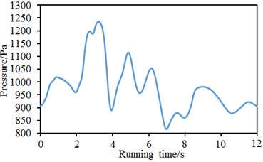
a) Nose tip of train head
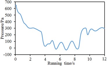
b) Nose tip of train tail
Fig. 14Contours for the pressures of the high-speed passing through the tunnel

a)0.2 s

b)4.2 s
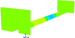
c)7.2 s
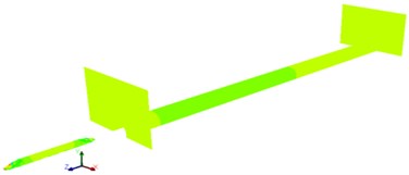
d)12.0 s
Pressure fluctuations of 6 observation points on tunnel surface were extracted, as shown in Fig. 15. Pressure fluctuation at this speed was similar to that at the speed of 250 km/h. However, maximum pressures were different at the two speeds. The maximum pressure was 300 Pa at the speed of 150 km/h and 821 Pa at the speed of 250 km/h. Similarly, the pressure fluctuations of observation point A and F were different from those of other observation points because the two observation points were at the tunnel entrance and exit respectively and free from the impact of superposition of compression and expansion waves. The pressure waves of the other four observation points were similar and only peak and valley values appeared at different times.
Fig. 15Comparison of pressure waves of 6 observation points
3.4. Pressure waves in near-field and far-field at the speed of 350 km/h
In the tunnel, the high-speed train ran at the speed of 350 km/h and observation points were in the same positions. Pressure waves at the nose tip of train head and tail were computed, as shown in Fig. 16. As displayed from Fig. 16(a), pressure fluctuation at the nose tip of train head was severe and showed two valley values and three peak values in the running process of high-speed train. When running time was 2.3 s and 3.5 s, the valley pressures of high-speed train were 3890 Pa and 4870 Pa respectively. When running time was 1.2 s, 2.8 s and 3.8 s, the peak pressures of high-speed train were 6710 Pa, 5690 Pa and 5570 Pa respectively. The difference value between the maximum pressure and the minimum pressure was 2820 Pa. As displayed from Fig. 16(b), pressure sharply decreased with the increase of running time when running time was less than 1.6 s. However, pressure showed two obvious valley values including –1120 Pa and –610 Pa when running time was more than 1.6 s. The contours for the pressures of high-speed train passing through the tunnel at the speed of 350 km/h were extracted, as shown in Fig. 17. Fig. 17 presented the contours for the pressures of high-speed train which did not enter the tunnel, just entered the tunnel, ran in the middle of the tunnel and pulled out of the tunnel. Similar to the change rule in Fig. 11, pressure on tunnel surface presented dynamic changes due to the impact of compression and expansion waves.
Fig. 16Pressures at the nose tip of train head and tail
a) Nose tip of train head
b) Nose tip of train tail
Fig. 17Contours for the pressures of the high-speed train passing through the tunnel
a)0.2 s

b)1.8 s

c)3.0 s
d)5.0 s
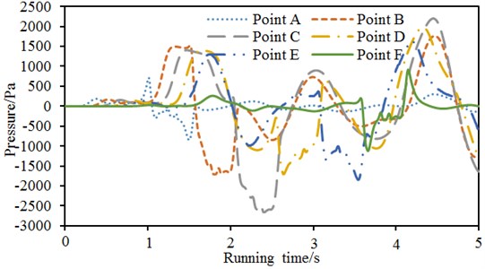
Pressure fluctuations of 6 observation points on tunnel wall were extracted, as shown in Fig. 18. Pressure fluctuation at this speed was similar to that at the speed of 250 km/h. However, maximum pressures were different at the two speeds. The maximum pressure was 2200 Pa at the speed of 350 km/h and 821 Pa at the speed of 250 km/h. Similarly, the pressure fluctuations of observation point A and F were different from those of the other observation points because the two observation points were at the tunnel entrance and exit and free from the impact of superposition of compression and expansion waves. Pressure waves of other four observation points were similar and only peak and valley values appeared at different times.
Fig. 18Comparison of pressure waves of 6 observation points
4. Impacts of parameters on train surface pressures
When a high-speed train passed through a tunnel, the blocking ratio, tunnel length and running speed will cause serious impacts on maximum and minimum pressures of the train surface. The rules can be obtained through comparison and analysis based on computation of train tunnel models under different parameters.
4.1. Running speed
Tunnel length and blocking ratio were kept unchanged. The train running speed was changed from 250 km/h to 500 km/h, and the step length was 50 km/h. Maximum and minimum pressures on the train surface under each work condition were computed, as shown in Fig. 19. It is shown in the figure that obvious linear relations were between the pressures on the train surface and the running speed. The maximum and minimum pressures gradually increased with the increased running speed as the increase of running speed will improve the acting force of airflows on the train surface. In addition, at the same running speed, the maximum and minimum pressures on the train surface increased with the increased blocking ratio as the increase of blocking ratio will improve effects of compression waves and expansion waves when the train entered and left the tunnel.
Fig. 19Pressures on the train surface under different running speeds
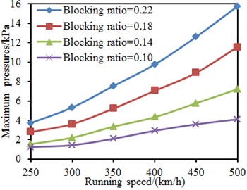
a) Maximum pressures
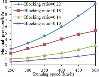
b) Minimum pressures
4.2. Blocking ratio
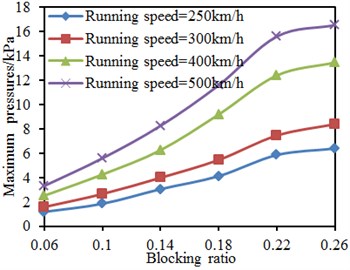
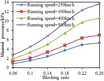
Running speed and tunnel length were kept unchanged. The blocking ratio was changed from 0.06 to 0.26, and the step length was 0.04. Maximum and minimum pressures on the train surface under each work condition were computed, as shown in Fig. 20. It is shown in the figure that: when the blocking ratio was smaller than 0.22, obvious linear relations were between the pressures on the train surface and the blocking ratio; pressures gradually increased with the increased blocking ratio as the increase of blocking ratio will improve effects of compression waves and expansion waves when the train entered and left the tunnel. However, when the blocking ratio was more than 0.22, it did not cause obvious impacts on maximum and minimum pressures of the train surface as the blocking ratio was very large at this moment and the effects of compression waves and expansion waves generated when the train entered and left the tunnel will not be improved. Under the same blocking ratio, the maximum and minimum pressures on the train surface gradually increased with the increased running speed as the increase of running speed will improve acting forces of airflows on the train surface.
4.3. Tunnel length
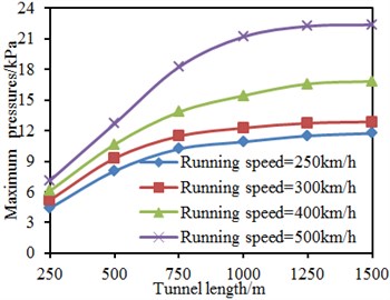
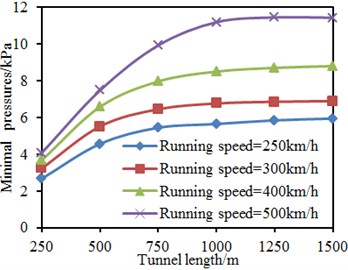
Running speed and blocking ratio were kept unchanged. The tunnel length was changed from 250 m to 1500 m, and the step length was 250 m. Maximum and minimum pressures on the train surface under each work condition were computed, as shown in Fig. 21. It is shown in the figure that: when the tunnel length was smaller than 750 m, linear relations were between the pressures on the train surface and the tunnel length; pressures gradually increased with the increased tunnel length as the train will generate many times of overlaying of expansion waves and compression waves when it entered and left the tunnel with the increased tunnel length. However, when the tunnel length was more than 750 m, the tunnel length did not generate obvious impacts on maximum and minimum pressures of the train surface as the tunnel length was very large at this moment and overlaying effects of compression waves and expansion waves generated when the train entered and left the tunnel were not improved any longer. Under the same tunnel length, the maximum and minimum pressures on the train surface gradually increased with the increased running speed as the increase of running speed will obviously improve acting forces of airflows on the train surface.
Fig. 20Pressures on the train surface under different blocking ratios
a) Maximum pressures
b) Minimum pressures
Fig. 21Pressures on the train surface under different blocking ratios
a) Maximum pressures
b) Minimum pressures
5. Positions of the maximum positive and negative pressures in the tunnel
As shown in Fig. 18, the maximum positive and negative pressure values of air pressure in the tunnel were 2200 Pa and –2700 Pa and appeared at the observation point C when the train passed through the tunnel at the speed of 350 km/h. The observation point C was 100 m away from the tunnel inlet. Based on this observation point, the impact of compression and expansion waves in the tunnel was analyzed, as shown in Fig. 22. As displayed from Fig. 22, tilted black solid lines were the propagation path of compression wave in the tunnel; black dotted lines were the propagation path of expansion wave; tilted green solid lines were the motion track of train head and tail. Qualitatively, the air pressure in this position increased when the compression wave caused by train head entering the tunnel inlet was spread to the observation point; air pressure in this position decreased when the expansion wave of train tail was spread to the observation point. Pressure in this position rose suddenly when train head passed through the observation point and decreased all of a sudden when train tail passed through the observation point. Other fluctuations in the course of pressure should be the result of back-and-forth transmission and superposition of compression wave or expansion wave at the inlet. Therefore, the wave peak of positive pressures in different positions of Fig. 22 at the time of 1 to 2 s resulted from compression wave of inlet caused by train head entering the tunnel and terminated when the expansion wave of train tail passed through the observation point. The closer the observation point was to the inlet, the more square positive pressure wave would be. When the observation point was close to the rear, the shape of positive pressure wave tended to be flat due to the attenuation of wall friction and the decline of peak values. The wave valley like an inverted-trapezoid groove in Fig. 22 was caused by air disturbance resulting from high-speed train passing through observation points.
Fig. 22Course of pressure at the place 100 m away from the tunnel inlet
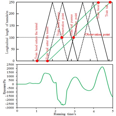
As shown in Fig. 22, the maximum positive pressure appeared due to the compression wave caused by train head entering the tunnel. The impact of compression wave would continue till the expansion wave caused by train tail entering the tunnel was spread to observation points. Therefore, the peak value of positive pressure waves caused by the first compression wave around the tunnel inlet was the largest and the width of compression wave was related to train length. In addition, pressure would rise momently when train head passed through observation points. If the position of observation points was within the width of the first compression wave (in the continuous process of compression wave), a small positive pressure value would be superimposed on the peak pressure of positive pressure waves, as shown in Fig. 22. As a result, the peak value of positive pressures caused by the train passing through the tunnel should appear when the train entered the tunnel. Pressure change caused by the train passing through observation points was superimposed on the propagation of pressure waves at the tunnel entrance and superimposed effect. In addition, large negative pressure would be produced when the train passed through the tunnel. Thus, the position of the maximum negative pressure in the tunnel could be obtained if the position of the maximum wave valley caused by pressure waves at the inlet could be determined. Qualitatively, it could be considered that the arrival of compression wave led to the rise of local air pressure and the arrival of expansion wave gave rise to the decrease of local air pressure. In this case, continuous compression waves resulted in the constant rise of local air pressure and continuous expansion waves contributed to the constant decrease of local air pressure. A peak and valley of pressure waves would appear between compression and expansion waves. According to this analysis and the propagation rule of compression and expansion waves at the inlet, the position of the maximum air pressure in the tunnel could be determined. For instance, the propagation of pressure wave at the tunnel entrance and the running track of the train were shown in Fig. 23 when the train ran at the speed of 350 km/h. In Fig. 23, black solid lines were the propagation path of compression wave; black dotted lines were the propagation path of expansion wave; green solid lines were the motion track of train head and tail.
Fig. 23Possible position of the maximum positive pressure in the tunnel
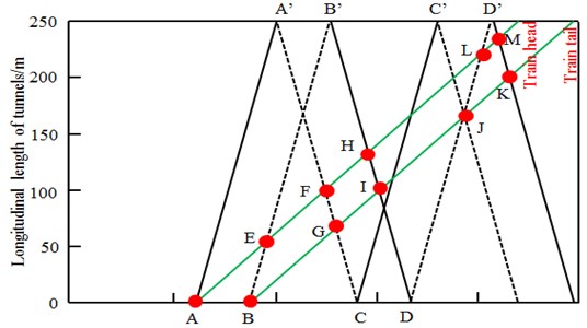
Fig. 24Positions of the maximum negative pressure in the tunnel at different speeds
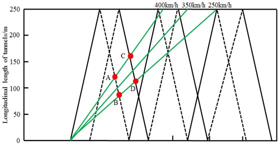
In Fig. 23, A-A' was compression wave caused by the entrance of train head into the tunnel; B-B' was expansion wave caused by the entrance of train tail into the tunnel; a peak of pressure waves should appear in the area between the two lines. Small-amplitude positive pressure would be aroused based on the peak of pressure waves when train head passed through this area. Therefore, the maximum value of air positive pressure might appear in the area ABE of Fig. 23. In Fig. 23, A'-C was the propagation path of expansion wave converted by the compression wave of train head at the tunnel outlet; the nearby area together with B-B' was the expansion wave; pressure kept decreasing till the expansion wave of train tail converted to compression wave B'-D at the tunnel outlet. Therefore, a valley value of pressure would appear between A'-C and B'-D. At this time, air pressure in this position would further decrease based on the wave valley of pressure if the train passed, which thus formed a valley value of negative pressure. As a result, the valley value of air negative pressure would appear in the area FGIH of Fig. 23. The position of valley value could be estimated from Fig. 23 though the specific position of the valley of pressure wave caused by the pressure wave of wall effect was unknown. The above analysis only involved the first compression wave, the first expansion wave and the superposition of their first converted waves. If the tunnel was very long, it was possible to present the peak value of positive pressures caused by the superposition of more continuous compression waves or the peak value of negative pressures caused by the superposition of more continuous expansion waves. For example, the area JKLM of Fig. 23 also satisfied the conditions of valley of pressure wave. If the passing of train head through the tunnel was taken as the benchmark, wave valley might be produced in the area ABCD of Fig. 24 when the train passed through the tunnel at the speed of 250 km/h to 400 km/h. At this time, the maximum negative pressure might be produced when the train passed through this area. The position of the maximum negative pressure could be estimated according to the time and speed of this area when the train ran.
6. Conclusions
1) In the open air, pressure fluctuation at the nose tip of train head was severe and showed two obvious valley and peak values. The difference value between the maximum pressure and the minimum pressure was only 125 Pa. Pressure at the nose tip of train tail did not present obvious fluctuations. Pressure at the train head was obviously more than that at the train tail. For different observation points, the peak and valley values of far-field pressures only showed translation with the increased running time.
2) In the tunnel, pressures at the nose tip of train head showed obvious peak and valley values and were far more than those in the open air. For different observation points, the peak and valley values of far-field pressures did not simply present translation with the increased running time, which indicated that there was wall effect in the tunnel.
3) In the tunnel, numerically computational and experimental results of pressure waves showed a good consistency, which showed that the model for the high-speed train passing through the tunnel in this paper was right. In addition, the absolute values of the maximum positive and negative pressures of the high-speed train in the near and far fields obviously increased with the increased running time.
4) The pressure fluctuation caused by the passing high-speed train in the tunnel was the superposition of the pressure wave of inlet effect and air disturbance caused by the passing the train. The size of local air pressure was related to tunnel length, train length and speed.
5) The peak value of positive pressures in the tunnel appeared when the train entered the tunnel. The valley value of negative pressures in the tunnel would appear in the area where the expansion wave of train head was superimposed with the compression wave of train tail. According to tunnel length, train length and speed, the specific positions where the peak and valley values of positive and negative pressures appeared could be approximately obtained. If the tunnel was very long, it was possible to present the peak value of positive pressures caused by the superposition of more continuous compression waves or the peak value of negative pressures caused by the superposition of more continuous expansion waves.
References
-
Cross D., Hughes B., Ingham D., et al. Enhancing the piston effect in underground railway tunnels. Tunnelling and Underground Space Technology, Vol. 61, 2017, p. 71-81.
-
Pindado S., Cubas J., Sorribes Palmer F. On the analytical approach to present engineering problems: photovoltaic systems behavior, wind speed sensors performance, and high-speed train pressure wave effects in tunnels. Mathematical Problems in Engineering, 2015, https://doi.org/10.1155/2015/897357.
-
Yoon T. S., Lee S., Hwang J. H., et al. Prediction and validation on the sonic boom by a high-speed train entering a tunnel. Journal of Sound and Vibration, Vol. 247, Issue 2, 2001, p. 195-211.
-
Suzuki M. Unsteady Aerodynamic Force Acting on High Speed Trains in Tunnel. Quarterly Report of RTRI, Vol. 42, Issue 2, 2001, p. 89-93.
-
Fukuda T., Ozawa S., Masanobu I., et al. Distortion of compression wave propagating through very long tunnel with slab tracks. JSME International Journal Series B Fluids and Thermal Engineering, Vol. 49, Issue 4, 2006, p. 1156-1164.
-
Luo J. J., Ji H. D. Study on changes of pressure waves induced by a high-speed train entering into a tunnel with hood. Journal of the China Railway Society, Vol. 33, Issue 9, 2011, p. 114-118.
-
Liu F., Yao S., Liu T. H., Zhang J. Analysis on aerodynamic pressure of tunnel wall of high-speed railways by full-scale train test. Journal of Zhejiang University (Engineering Science), Vol. 50, Issue 10, 2016, p. 2018-2024.
-
Zhang F. Y., Cheng S. Development of wireless data acquisition system in real vehicle passing tunnels during aerodynamic tests. Journal of Railway Science and Engineering, Vol. 13, Issue 7, 2016, p. 1401-1406.
-
Huang Y., Wei G. A. O., Chang Nyung K.-I.-M. A numerical study of the train-induced unsteady airflow in a subway tunnel with natural ventilation ducts using the dynamic layering method. Journal of Hydrodynamics, Ser. B, Vol. 22, Issue 2, 2010, p. 164-172.
-
Dong H., Ning B., Cai B., et al. Automatic train control system development and simulation for high-speed railways. IEEE Circuits and Systems Magazine, Vol. 10, Issue 2, 2010, p. 6-18.
-
Gupta S., Van Den Berghe H., Lombaert G., et al. Numerical modelling of vibrations from a Thalys high speed train in the Groene Hart tunnel. Soil Dynamics and Earthquake Engineering, Vol. 30, Issue 3, 2010, p. 82-97.
-
Nejati H. R., Ahmadi M., Hashemolhosseini H. Numerical analysis of ground surface vibration induced by underground train movement. Tunnelling and Underground Space Technology, Vol. 29, 2012, p. 1-9.
-
Lopes P., Costa P. A., Ferraz M., et al. Numerical modeling of vibrations induced by railway traffic in tunnels: From the source to the nearby buildings. Soil Dynamics and Earthquake Engineering, Vol. 61, 2014, p. 269-285.
-
Juraeva M., Lee J., Song D. J. A computational analysis of the train-wind to identify the best position for the air-curtain installation. Journal of Wind Engineering and Industrial Aerodynamics, Vol. 99, Issue 5, 2011, p. 554-559.
-
Jia Y. X., Yang Y. G., Mei Y. G. Characters of pressure wave caused by high-speed trains passing tunnels based on 1D non-homentropic flow model. Journal of Mechanical Engineering, Vol. 50, Issue 24, 2014, p. 106-114.
-
Mei Y. G., Zheng C. Y., Zhou C. H., Jia Y. X., Wu M. Research on the actual discomfort when a single train passes through a super long tunnel. Journal of Mechanical Engineering, Vol. 51, Issue 14, 2015, p. 100-107.
-
Bell J. R., Burton D., Thompson M., et al. Wind tunnel analysis of the slipstream and wake of a high-speed train. Journal of Wind Engineering and Industrial Aerodynamics, Vol. 134, 2014, p. 122-138.
-
Xu J. L., Sun J. C., Mei Y. G., Wang R. L. Numerical simulation on crossing pressure wave characteristics of two high-speed trains in tunnel. Journal of Vibration and Shock, 2Vol. 16, Issue 35, 3, p. 184-192.
-
Li R. X., Yuan L. Pressure waves in tunnels when high-speed train passing through. Journal of Mechanical Engineering, Vol. 50, Issue 24, 2014, p. 115-121.
Cited by
About this article

