Abstract
With the continuously increased speed of the high-speed train, the lateral aerodynamic performance of high-speed trains has attracted more and more attention. Under strong crosswinds, the aerodynamic performance of trains deteriorate and air drag, lift and lateral forces borne by trains quickly increase, which has an impact on the lateral stability of trains and even leads to train derailment. This paper adopted computational fluid dynamics theory to establish an aerodynamic model for a high-speed train, computed aerodynamic forces and moments acting on the high-speed train and obtained the unsteady flow field of the high-speed train. In the meanwhile, this paper combined with multi-body system dynamics theory to establish a system dynamics model for the train and analyzed the safe aerodynamic performance of the high-speed train under cross winds. Computational results showed: Under cross winds, the aerodynamic performance of the high-speed train had a random fluctuation. When wind direction angle was 90°, aerodynamic forces (drag, lift and lateral forces) and moments (overturning moment, shaking moment and nodding moment) borne by the high-speed train were the largest; train speed was a main factor affecting the size of positive pressures of train and cross wind velocity had no obvious impacts on the positive and negative pressures of train body; the aerodynamic forces and moments of the high-speed train had a random fluctuation within a certain range with time; the frequency for the peak value of power spectral density of lateral forces of head train was within 25 Hz and the peak value of power spectral density was the largest when the main frequency was 1.6 Hz; the frequency for the peak value of power spectral density of overturning moment of head train was within 20 Hz and main frequency was 0.57 Hz. When the cross wind speed was 15 m/s, all safety indexes of the high-speed train running at the speed of 250 km/h were within the range of limited values and satisfied design requirements. Aerodynamic performance of the high-speed train with the suction chamber under the cross wind was computed and compared with original results. Aerodynamic force and force moments of the high-speed train under cross wind will be reduced obviously and running safety of the high-speed train can be improved through application of the suction chamber.
1. Introduction
With the continuously increased speed of the high-speed train, the lateral aerodynamic performance of high-speed trains has attracted more and more attention. Under strong cross winds, the aerodynamic performance of trains deteriorate and air drag, lift and lateral forces borne by trains quickly increase, which has an influence on the lateral stability of trains and even leads to train derailment. Researched shows that train derailment or overturn is likely to take place when train speed reaches 200 km/h and cross wind velocity is more than 30 m/s [1, 2]. To study the aerodynamic load characteristics and running safety of high-speed trains under cross winds, scientific researchers have made a lot of work. Khier [3] studied the structure of flow field around train body under different wind direction angles and found that vortex structures around the train was related to wind direction angle. Baker [4, 5] has conducted a lot of research work in wind tunnel experiments and real train tests and studied the steady and transient aerodynamic forces acting on various types of trains under cross winds. Suzuki [6] studied the aerodynamic response of a typical train running on a bridge and embankment through wind tunnel experiments. Diedrichs [7] used experimental and numerical simulation methods to study the external flow field of ICE2 tractor running on an embankment with a height of 6m. Numerical simulation results were consistent with test results. Results showed that the aerodynamic performance of train running on the leeward side of embankment deteriorated more than that running on the windward side of embankment. References [8-10] studied the dynamic response and running safety domain of the high-speed train under cross winds. Gao established the overturning stability of train in the track and train body on the bogie under the action of steady and transient loads according to the balance theory of static moment [11]. Tan analyzed the structure of flow field around the high-speed train under cross winds and obtained the change relationship between cross wind velocity, train speed and aerodynamic forces [12]. Wang used the test results of impact of cross winds on the aerodynamic response of motor trains to obtain the aerodynamic lift, lateral force and side rolling moment of the high-speed train under cross winds and applied SIMPACK software to analyze the straight-line running dynamics performance and passing performance of the high-speed train under cross winds [13-14]. Liu studied the running safety characteristic of the high-speed train under the action of unsteady aerodynamic forces under cross winds based on large eddy simulation (LES) method and SIMPACK software [15, 16]. Song combined ANSYS with SIMPACK software to study the impact of cross winds on the running safety of train running in a straight line [17]. Trainrarini took advantage of linear panel method and SIMPACK software to study the fluid-solid coupling vibration of train [18]. The research of references [19-20] showed that the value of safety indexes computed by using unsteady aerodynamic loads was more than that computed by using steady aerodynamic loads. Therefore, it was very important to study the unsteady aerodynamic characteristic and safety of the high-speed train under cross winds.
With the advantages of RANS and LES, detached-eddy simulation (DES) method has been applied to simulate the transient flow field around trains in recent years. Computational results are basically consistent with experimental results [21-23]. This paper combined the aerodynamics of the high-speed train with system dynamics to study the transient aerodynamic response and safety of the high-speed train under cross winds. Firstly, this paper established a numerically computational model for the aerodynamics of a high-speed train, adopted DES method to numerically compute the flow field around the train and conducted a detailed analysis on the unsteady response of aerodynamic loads borne by the high speed train and the unsteadiness of structure of flow field around the train. Then, this paper established a multi-body system dynamics model for the high-speed train, took aerodynamic loads as external loads, loaded them to the multi-body system dynamics model for computation, and studied the impact of cross winds on the safety of the aerodynamic performance of the high-speed train.
2. Computational method of the aerodynamic performance of trains under cross-winds
DES method based on Menter - SST two-equation turbulence model was adopted to solve Navier-Stokes equation. According to the basic thought of DES, RANS was adopted at the boundary layer near wall surface, and turbulence model was used to simulate small-scale fluctuations. In the area far away from object surface, LES was adopted to simulate the motion of detached vortexes. DES equation based on Menter - SST was:
wherein: is time; is density; is turbulent kinetic energy; is directional coordinate; 1, 2, 3 is length, width and height respectively; is the velocity component of airflow; is the generation item of turbulent flow; , , , , are empirical constants; is the dissipation rate of turbulence ratio; is turbulence scale parameter, ; is switch function which represented the minimum distance between vortex and wall surface. In the area close to the wall, is close to 1 and model is similar to - model. Near the edge of the boundary layer, is close to 0 and model transformed into - model. is the viscosity coefficient of laminar flow; is the viscosity coefficient of vortexes:
where is the absolute value of vortexes, . The mixed function was:
wherein, is the minimum distance between the first layer of grids and object surface.
In DES method, is replaced by . is the longest side length of grid cells. Constant is . Constant terms are and . In this case, value is quite large and turbulent kinetic energy is limited at the boundary layer close to object surface. is much less than the scale of grid cells. SST turbulence model worked and RANS was adopted. In the area far away from object surface, value was very small. When increased and was more than , the model after change acted as the sub-grid Reynolds stress model of LES.
3. Computational model for the aerodynamic performance of trains under cross-winds
3.1. Aerodynamic model
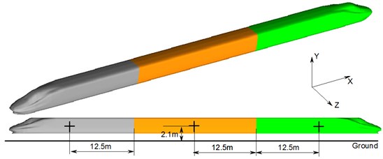
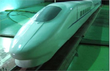
High-speed trains are a complex, long and thin structure. There will be a large amount of computation if numerical simulation is conducted for the flow field of a whole train. Therefore, we have used the model with scale 1:8 as the computational model in order to compare the results with those of the wind tunnel test. Keeping a certain distance from head train, the structure of flow field in the middle of a train is basically stable. This paper adopted a train model with three-train formation including head train, mid train and tail train. Head and tail trains had the same shape. In the meanwhile, the train was simplified into a geometry composed of smooth surface to avoid a large number of grids, irrespective of detail characteristics of pantographs, bogies, doorknobs and so on. This paper took a CRH2 motor train as the studied object and adopted three-train formation including head train, mid train and tail train. The simplified model for the high-speed train was shown in Fig. 1. The size parameters of the train were: 9.5 m long, 0.45 m wide and 0.46 m high. The streamline of head train was 1.1 m long.
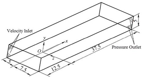
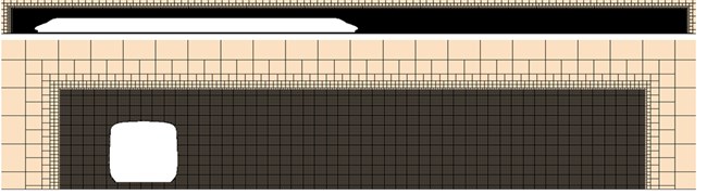
Computational domain and boundary conditions were shown in Fig. 2. On the top of the domain were symmetrical boundary conditions. At the bottom of the computational domain was ground which was set as slip wall. Slip velocity was the running speed of train to simulate ground effect. The surface of train was set as no-slip wall. The nose tip of head train of the high speed train was more than 1 times of train length (at a distance of 12.5 m) away from the velocity inlet right ahead the train; the nose tip of tail train was greater than 2 times of train length (at a distance of 28 m) away from pressure outlet right behind the train; the computational domain was 5 m high; the velocity inlet was 5m away from the longitudinal center line of train; the pressure outlet was 7.5 m away from the longitudinal center line of train.
Fig. 1Geometric model of the high-speed train
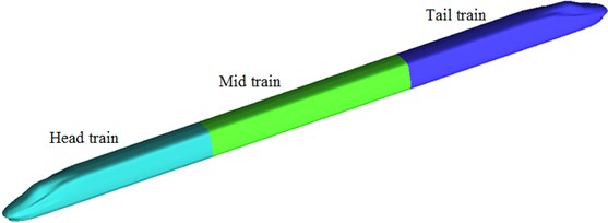
Fig. 2Computational domain of the high speed train
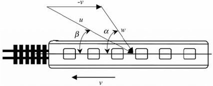
In the model, the principle of resultant winds was adopted to simulate the wind velocity of inlet, as shown in Fig. 3. Resultant wind velocity was obtained through considering the train as static and completing the vector resultant of environmental wind velocity and the reverse speed of train speed. was side slip angle. Research results showed that such an approximate processing method would not produce large errors in general [10].
Fig. 3Principle of resultant wind velocity
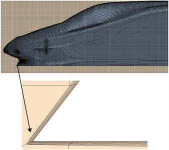
Trimmer grid was adopted to divide the grids of computational domain of the high speed train. Grids of the boundary layer on the surface of the high speed train were divided. Meanwhile, the area of grid refinement was set around the high-speed train, as shown in Fig. 4. The maximum grid size on the surface of train was 10 mm. The maximum grid size of spatial object was 180 mm. The maximum size of volume grids in the refinement area around the train was 5 mm. The local space grid of the high-speed train was shown in Fig. 5. There were 10 million grids in the computational model, and the computational result of the flow field was not related to the material property of the high-speed train.
Fig. 4Refinement area of computational domain
Fig. 5Schematic diagram for computational grids of the high-speed train
a) The whole train
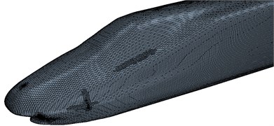
b) Head train
c) Grids of the boundary layer
3.2. Multi-body system dynamics model
The high-speed train is deemed as a multi-rigid body system. Dynamic model of each train is composed of 15 components including 1 train body, 4 wheel sets, 2 frameworks, and 8 steering arms. Displacement vector of the high-speed train can be expressed as follows:
wherein, , , and are the displacement vectors of train body, framework, wheel sets and axle box. Letters in subscript brackets represent the number of corresponding components. Train-track coupling dynamic equations could be established as follows:
where is mass matrix; is damping matrix; is rigidity matrix. and are equivalent forces caused by track irregularity and aerodynamic forces caused by two high-speed trains passing by each other [24, 25]. , , , , and are aerodynamic resistance, horizontal aerodynamic force, aerodynamic lift force, overturning moment, nodding moment and head shaking moment of the high-speed train. It is found in these formulas that aerodynamic force and force moments can be obtained after the displacement vector of the high-speed train was solved. Co-simulation of FLUENT and SIMPACK should be conducted to compute the displacement vector of the high-speed train under aerodynamic loads.
In general, FLUENT and SIMPACK are used independently regarding aerodynamic problems and dynamic problems of the high-speed train respectively. However, aerodynamics and system dynamics of the high-speed train are closely coupled. Therefore, it is necessary to set up a co-simulation environment which combines FLUENT and SIMPACK, make use of advantages of software and conduct in-depth analysis on dynamic behaviors of the high-speed train under aerodynamic loads. Coupling problems between aerodynamics and system dynamics are solved based on co-simulation of FLUENT and SIMPACK according to the following ideas: An interface program is used to connect an aerodynamic solver to a system dynamic solver; FLUENT is taken as a computational engine of aerodynamics in the interface program and used to provide aerodynamic loads of the train under current posture in real time; the interface program then transmits aerodynamic loads to SIMPACK.
Fig. 6Multi-body system dynamics model of the high-speed train
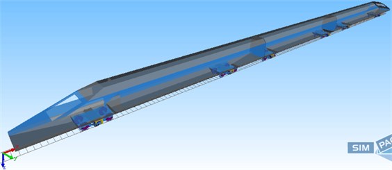
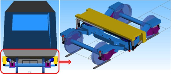
Firstly, SIMPACK was used to establish a multi-body dynamic model of the high-speed train with three train formations including a head train, a mid-train and a tail train. In order to show real performance of the high-speed train as accurately as possible and make computation and analysis convenient, the rational hypotheses were made during establishing the multi-body dynamic model of the high-speed train: 1) Front and rear bogies of the same train body had the same structure and parameters, while they were symmetrical to the train body center; 2) Components including bogies, framework, wheel set and train body were deemed as rigid bodies, while other elastic deformation was not considered; 3) Only the irregular excitation of steel tracks was taken into account, where its elastic deformation was not taken into account. Therefore, the high-speed train system can be deemed as a multi-rigid body system, where the dynamic model of each train is composed of 15 components including 1 train body, 4 wheel sets, 2 frameworks and 8 steering arms. The rigid body, framework and wheel set have 6 degrees of freedom respectively, namely vertical direction, longitudinal direction, horizontal direction, head shaking, nodding and lateral rolling; the steering arm has 1 degree of freedom, namely nodding; the dynamic model of each train has 50 degrees of freedom, and the dynamic model of the complete train has 150 degrees of freedom. Each structure of a train system is expressed by equivalent spring, damping and mass block; a distributed track model is adopted for the track system [24]. The multi-body dynamic model of the high-speed train was established according to the following processes: After necessary parameters of the high-speed train were obtained, the train system was firstly simplified by rational hypotheses. Specifically, the definition of basic attributes of each rigid body, definition of three-dimensional geometric shape, determination of hinging and applied force elements as well as sensors, constraints, and topological relations of multi-body elements should be conducted. Train treads are mainly classified into LMA, LM, S1002 and S1002G. The wheel-track contact relations were very different after matching between four treads and the steel track of 60 kg/m (CN60). Limited by tread tapers of different tread types, horizontal and vertical accelerations of the train body with LMA treads were the minimum; maximum values were corresponding to S1002G treads, where horizontal accelerations of the train body were more than vertical accelerations. LMA took full account of nonlinearity of wheel-track contact, creep linearity and non-linear suspension. This indicates that the train body with LMA treads had a high steadiness, and vertical steadiness of the train was better than horizontal steadiness. Based on above hypotheses and analysis, the multi-body dynamic model of the high-speed train was established, as shown in Fig. 6.
Fig. 7Irregular track spectrums of the high-speed train
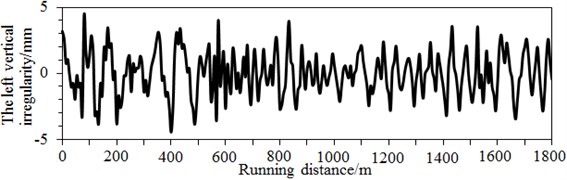
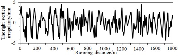
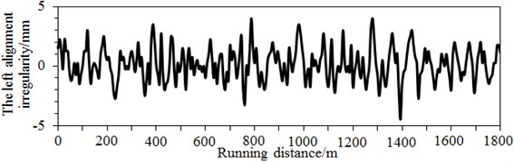
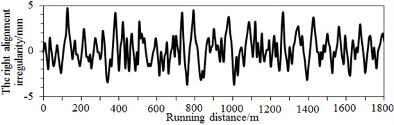
In the ideal status, the steel track is fixed and has a smooth, flat and straight surface. However, in practice, the steel track may suffer from deviation caused by geometric shapes, dimensions and spatial positions. Steel track surface defect, namely geometric parameter deviations caused by a track in horizontal and vertical directions relative to the rational flat and straight track, is called as the track irregularity. In the paper, the vertical and alignment irregularity spectrums of the track in Fig. 7 were input into the multi-body dynamic model of the high speed train.
Through co-simulation of FLUENT and SIMPACK, aerodynamic distribution forces of the high-speed train under crosswinds could be obtained. Then, each train was deemed as a rigid body. According to principles of force translation and equivalence, distributed pressures acting on the train surface were simplified to a point of the train body. Therefore, aerodynamic resistance, horizontal aerodynamic force, aerodynamic lift force, overturning moment, nodding moment and head shaking moment acting on each train were obtained. Simplified centers of each train are shown in Fig. 8. The train body centroid was selected as the simplified center. Integration was conducted to the distributed pressure acting on the train surface, so equivalent concentrated force and force moment acting on the train body were obtained.
Fig. 8Simplified center of each train body of the high-speed train
4. Flow field around the high-speed train
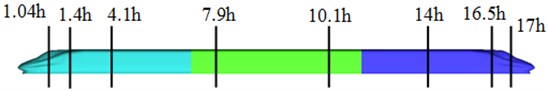
8 planes vertical to train body were selected along the longitudinal direction of the high-speed train, as shown in Fig. 9. Texts on the cross-section were their distance with the nose tip of head train and h represented the height of train.
Fig. 9Schematic diagram for cross-sections of the high speed train
In the published researches, constant wind velocities were often used as cross wind loads. However, it did not satisfy actual situations. Therefore, the paper considered using fluctuating wind velocities as the cross wind loads. Therefore, the constant wind velocity of 10 min was transformed into transient fluctuating wind velocities. In this paper, average wind velocities of 10 m/s, 15 m/s, 20 m/s, 25 m/s and 30 m/s under fluctuating wind velocities were adopted, respectively. It was shown in Fig. 7 that results under the running distance of 1800 m were simulated in this paper. As shown in Fig. 10, 24 simulation points were arranged within the distance of 1800 m, where the distance between every two simulation points was 75 m. The harmonic wave superposition method in MATLAB was used to achieve simulation of random wind fields. Kaimal spectrum was used as the wind velocity spectrum. Ground roughness was . Average wind velocity was 40 m/s. MATLAB computation which generated fluctuating wind velocities using the harmonic wave superposition method was conducted by the following processes: Firstly, wind velocity time-history parameters were set. Secondly, a target power spectrum was generated, and the fluctuating wind velocity time-history of point 1 was simulated. Finally, random phases of points 2-24 were computed based on point 1, and fluctuating wind velocity time-histories of points 2-24 were simulated. Therein, the fluctuating wind velocity time-history under the average wind velocity of 30 m/s was shown in Fig. 11. It was shown in the figure that natural wind fluctuations were serious, and the cross wind was not a constant value. Therefore, during studying aerodynamic performance of the high-speed train under the cross wind, using the constant wind velocity as the excitation load will seriously get deviated from actual situations.
Fig. 10Simulation points of fluctuating wind velocities
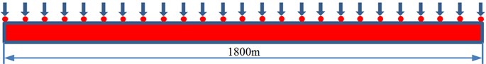
Fig. 11Fluctuating wind velocities at simulation points 1 and 24
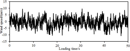
a) Simulation point 1
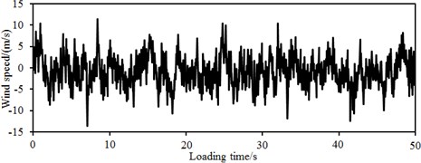
b) Simulation point 24
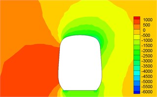
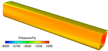
Fig. 12Contour for pressures of different cross-sections
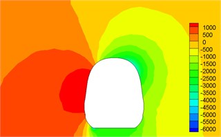
a)1.04 h
b)1.4 h
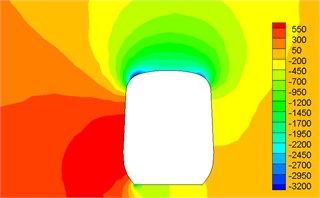
c)4.1 h
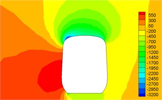
d) 7.9 h
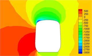
e)10.1 h

f) 14 h
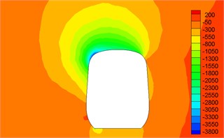
g)16.5 h
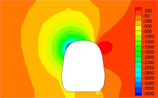
h)17 h
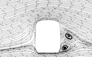
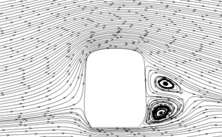
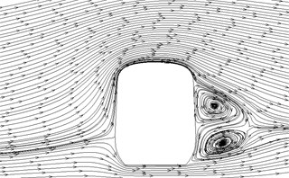
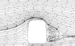
Fig. 12 displayed the contour for the pressure distribution of cross-sections shown in Fig. 9 when the high-speed train ran at the speed of 250 km/h and cross wind velocity adopted fluctuating wind velocity as the excitation load. Fig. 13 displayed the contour for velocity distribution of cross-section shown in Fig. 9 when the high-speed train ran at the speed of 250 km/h and cross wind velocity was 30 m/s. Fig. 14 displayed the diagram for velocity streamline of cross-sections shown in Fig. 9 when the high-speed train ran at the speed of 250 km/h and cross wind velocity was 30 m/s.
It could be seen from contours for pressures and velocities and velocity streamline of different cross-sections:
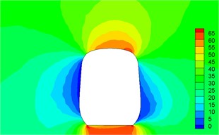
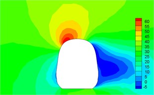
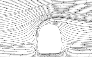
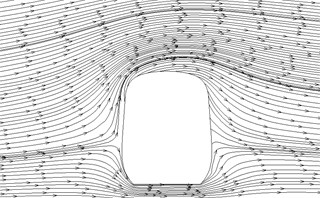
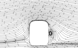
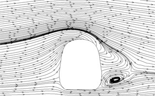
(1) Contour for the pressure of cross-section of head train showed: positive pressures were on the windward side, negative pressures were on the leeward side and the direction of lateral force of head train was the same with wind direction; as the cross-section was far away from the nose tip of head train, positive pressures on the windward side decreased and negative pressures on the leeward side also decreased. Therefore, lateral force in the part of streamline train head was more than that in the part of train body; the maximum flow velocity of streamline train head and body on the top of train partial to the leeward side; vortexes appeared on the leeward side of head train body.
(2) For two cross-sections on the mid train, positive pressures were on the windward side and negative pressures were on the leeward side so that the mid train bore lateral forces with the same wind direction; as cross-sections were far away from the nose tip of train head, pressure distribution and distribution of velocity magnitude on the two cross-sections were basically the same, which also proved the rationality of simplified model in this paper; the maximum flow velocity in the part of mid train body appeared in the circular arc transition from the train body on the leeward side to the top of mid train; two vortexes appeared on the leeward side of mid train body.
(3) For three cross-sections on the tail train, the windward side bore positive pressures and the leeward side bore negative pressures at 14 h of cross-section; the position at 16.5 h of cross-section basically bore negative pressures; at 17 h of cross-section, the circular arc transition from train top to the leeward side of train body bore positive pressures; other parts mainly bore negative pressures; the value of negative pressures on the windward side was very large so that tail train bore side force opposite to wind direction; the maximum flow velocity of tail train body appeared in the circular arc transition from train body on the windward side to the train top; the maximum flow velocity in the streamline part of tail train was on the windward side; two vortexes appeared on the leeward side of tail train.
(4) In the part of tail train and mid train close to tail train, contour for velocities had negative values, which showed the phenomenon of airflow reflux. Vortexes here were more than those in other parts.
Fig. 13Contour for velocities of different cross-sections
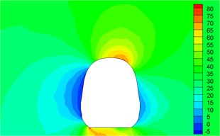
a)1.04 h
b)1.4 h
c)4.1 h
d) 7.9 h
e)10.1 h
f) 14 h
g)16.5 h
h)17 h
Fig. 14Streamline diagram of different cross-sections
a)1.04 h
b)1.4 h
c)4. 1 h
d) 7.9 h
e)10.1 h
f) 14 h
g)16.5 h
h)17 h
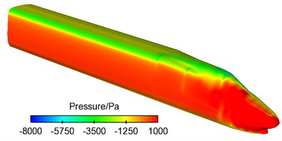
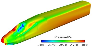
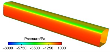
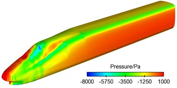
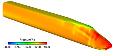
Fig. 15 displayed the contour for pressure distribution on the surface of train body when the high-speed train ran at the speed of 250 km/h and crosswind velocity was fluctuating wind velocity.
(1) Areas of the maximum positive pressures of the high-speed train were partial to the windward side of nose tip of head train of the train while areas of positive pressures of tail train were partial to the leeward side. Thus, it was clear that head and mid trains bore side forces which had the same direction with cross winds and tail train bore side forces opposite to the direction of cross winds.
(2) On the windward side of train body were mostly positive pressures. On the transition arc surface from the side of train to the top of train, positive pressures quickly decreased and changed into negative pressures. Train bodies on the leeward side of high-speed train were basically areas of negative pressures.
(3) The increase of positive pressures of head and tail trains was mainly affected by train speed. With the increase of running speed of train, its positive pressures increased most and negative pressures increased least. Under the same train speed, the positive pressures of head and tail trains increased a lot and negative pressures basically kept unchanged with the increase of cross wind velocity. Thus, it was clear that train speed was a main factor affecting the size of positive pressures of train and cross wind velocity had no obvious impacts on the positive and negative pressures of train body.
5. Analysis on the aerodynamic performance of the high-speed train under cross wind
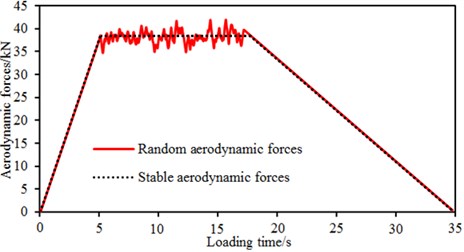
After flow field computation of the high speed train was complete, aerodynamic forces were simplified to the centroid, so loads acting on the multi-body dynamic model of the high speed train were obtained. In the reported researches, aerodynamic forces were basically simplified into stable loads and applied on the multi-body dynamic model of the high speed train. For example, Liu [26] applied stable loads in the multi-body dynamic model of the high speed train, so dynamic responses and safety indexes generated when the train ran at different velocities without and with cross wind were computed. However, using the stable load as the excitation and applying it to the multi-body dynamic model of the high speed train cannot satisfy actual situations. Therefore, in this paper, random loads and stable loads were applied to the high speed train respectively, so aerodynamic force and force moment can be computed for comparative analysis, as shown in Fig. 16. Therein, during 0-5 s, the aerodynamic force value was reached through linear loading, so running of the high speed train gradually tended to be stable. Aerodynamic forces acted within 5-18 s. Then, the force reached 0 through linear unloading.
Fig. 15Contour for pressures on the surface of the high-speed train
a) Windward side of head train
b) Leeward side of head train
c) Windward side of mid train
d) Leeward side of mid train
e) Windward side of tail train
f) Leeward side of tail train
Fig. 16Two different loading methods
5.1. Impact of wind direction angle on the aerodynamic performance of trains under stable aerodynamic forces
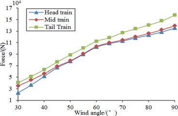
Firstly, aerodynamic performance of the high speed train under stable loads was computed based on the above model. To study the impact of different wind direction angles on the aerodynamic performance of train, an analysis was conducted through selecting different wind direction angles (30°, 45°, 60° and 90°) when the high-speed train ran at the speed of 250 km/h and cross wind velocity was fluctuating wind velocity. Fig. 17 displayed the curves of lift, lateral force, overturning moment and shaking moment of all train bodies changing with wind direction angle. As shown in Fig. 17, different wind direction angles had different impacts on the aerodynamic performance of train under the same wind velocity. Under the same wind velocity, the aerodynamic force (moment) was the largest and its safety performance was the poorest when wind direction angle was 90°. In addition, the overturning moment of the head train was the maximum because it was facing the airflow of the computational domain. As shown in Fig. 17(b), the lateral force of the head train was also the maximum, so it will cause the maximum overturning moment in the high-speed train.
Fig. 17Force and moment of all train bodies changing with wind direction angle
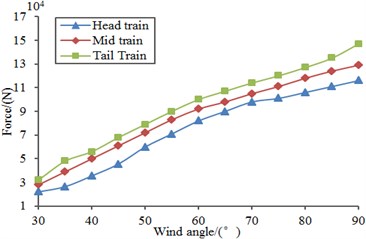
a) Lift
b) Lateral force
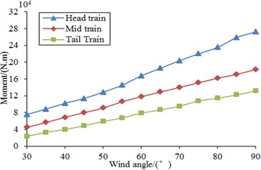
c) Overturning moment
d) Shaking moment
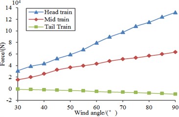
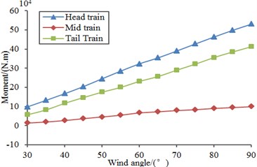
5.2. Impact of wind direction angle on the aerodynamic performance of trains under random aerodynamic forces
Similarly, based on the above computation model, random loads were applied to the model to compute aerodynamic force and force moment of the high speed train under different wind direction angles, as shown in Fig. 18. It was shown in the figure that aerodynamic force and force moment gradually increased with the increased wind direction angle as the cross wind loads acting on the high speed train will be larger when the wind direction angle was larger. In addition, compared with Fig. 17, we can find that aerodynamic force and force moment under the random loads were obviously different from those under stable loads. Therefore, random aerodynamic forces should be loaded during computing aerodynamic performance of the high speed train under cross wind.
Fig. 18Force and moment of all train bodies changing with wind direction angle
a) Lift
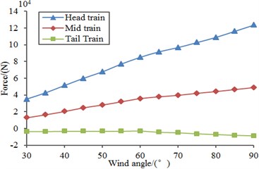
b) Lateral force
c) Overturning moment
d) Shaking moment
5.3. Impact of running speed on the aerodynamic performance of trains
The lateral force coefficient of the high-speed train was defined as follows:
where is the lateral force coefficient of train; is the lateral force value of train; is air density. This paper chose 1.225 kg/m3. is the running speed of train. is the maximum cross-section area (m2) of train.
Fig. 19 displayed a diagram for the comparison of lateral force coefficients when the high-speed train was at the cross wind velocity of 30 m/s. As displayed from the comparative analysis of Fig. 19 and Fig. 20, head train bore the maximum lateral force coefficient, followed by tail train and mid train. Under the same cross wind velocity, lateral force coefficients of all train bodies gradually decreased with the increase of running speed of train. Under the same running speed of train, lateral force coefficients of all train bodies increased a lot with the increased cross wind velocity. In addition, lateral force coefficients of all train bodies presented an approximate linear relationship with the increased cross wind velocity, as shown in Fig. 20.
The overturning moment coefficient of the high-speed train was defined as follows:
where is the overturning moment coefficient of train; is the overturning moment value of train. is air density. This paper chose 1.225 kg/m3. is the running speed (m/s) of train; is the maximum cross-section area (m2) of train; is the maximum lateral width of train.
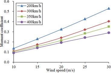
Fig. 21 displayed a diagram for the comparison of overturning moment coefficients when the high-speed train was under the cross wind velocity. Fig. 22 displayed a diagram for the comparison of overturning moment coefficients of head train under different cross wind speed. As shown in the comparative analysis of Fig. 21 and Fig. 22, head train bore the maximum overturning moment coefficient, followed by mid train and tail train. Under the same cross wind speed, overturning moment coefficients of all train bodies gradually decreased with the increased running speed of train. Under the same running speed of train, overturning moment coefficients of all train bodies gradually increased with the increased cross wind speed. In addition, overturning moment coefficients of all train bodies presented an approximate linear relationship with the increased cross wind speed, as shown in Fig. 22.
Fig. 19Lateral force coefficients of all train bodies
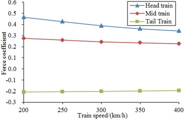
Fig. 20Lateral force coefficients under different cross wind speed
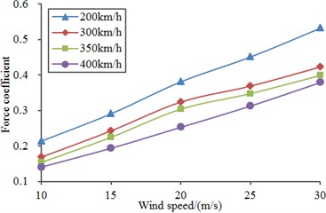
Fig. 21Overturning moment coefficients of all train bodies
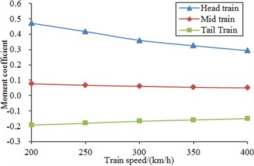
Fig. 22Overturning moment coefficients under different wind speed
5.4. Experimental verification of co-simulation model of the high-speed train
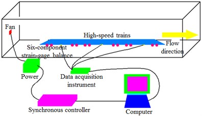
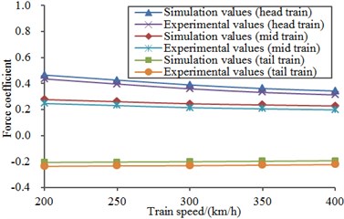
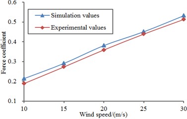
The experiment was conducted in an 8 m×6 m wind tunnel section. The wind tunnel was a closed series wind tunnel, where the cross section area of the experimental section was 8 m×6 m, the length was 15 m, and the steady wind speed scope was 30 m/s-120 m/s. In order to reduce impacts of the floor boundary layer, a floor device dedicated for the train experiment was installed in the experimental section. The upper surface of floor was 1.06 m away from the lower wall of wind tunnel. Front and rear edges of the floor were processed into a streamline type, so interference to airflows was reduced. The experimented train model was a metal frame structure. The external part was made of wood, so the model could have enough strength and rigidity and would not get deformed and generate obvious vibration during the experiment, so measurement accuracy could be guaranteed. The model scale was 1:8, and three train formations were adopted. The experimental model is shown in Fig. 23(a). Experimental test processes are shown in Fig. 23(b). Head and tail parts of the train were completely symmetric. The crosswind had a 90° wind direction angle. Measurement was conducted with a six-component strain balance which was used to test aerodynamic force and force moments of the train model. In the experiment, the horizontal wind speed was changed according to the numerical simulation. The longitudinal wind speed was changed within 200 km/s-400 km/h, so running working conditions of the high-speed train under different speeds could be simulated. Finally, experimental results were compared with numerical simulation results, as shown in Fig. 24. It is shown in Fig. 24 that experimental values were very close to numerical simulation values. Errors were caused by human and instrument errors in experiments. However, the maximum relative error between numerical simulation and experimental test was only 5 %. It is thus clear that the numerical model can completely replace experimental test in subsequent researches.
Fig. 23Experimental model and process of the high-speed train
a) Experimental model
b) Experimental processes
Fig. 24Comparison between experimental results and numerical simulation results
a) Lateral force coefficients of trains
b) Lateral force coefficients under different cross wind speed
5.5. Unsteady aerodynamic responses of the high-speed train under cross-winds
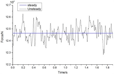
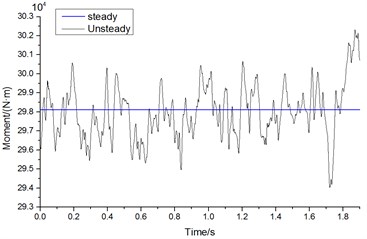
Computational results under different working conditions were analyzed to find that aerodynamic loads of the high-speed train had obvious unsteady characteristics and fluctuated around the mean value under cross winds. In addition, aerodynamic loads of head train were generally more than those of mid and tail trains. Head train was taken as an example. Fig. 25 displayed the curves of lateral force and overturning moment of head train changing with time when the high-speed train ran at the speed of 250 km/h and cross wind speed was fluctuating wind velocity. As shown in the comparison of Fig. 25, aerodynamic forces and moments of the high-speed train had a random fluctuation within certain limits with time. The lateral force of fluctuation changed from 123 kN to 127 kN and fluctuation range of overturning moment was approximately from 295 kN.m to 301 kN.m.
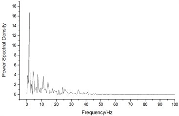
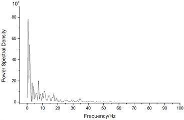
Fig. 26 displayed the power spectral densities of lateral force and overturning moment of head train when the high-speed train ran at the speed of 250 km/h and cross wind speed was fluctuating wind velocity. As shown in Fig. 26, the frequency for the peak value of power spectral density of lateral force of head train was within 20 Hz and the peak value of power spectral density was the largest, namely 16.8×10⁴ N2·Hz-1 when the main frequency was 1.6 Hz. The frequency for the peak value of power spectral density of overturning moment of head train was within 20 Hz and the peak value of power spectral density was the largest, namely 78.2×10⁴N2·Hz-1 when the main frequency was 0.57 Hz.
Fig. 25Curves of unsteady aerodynamic forces and moments of head train changing with time
a) Lateral force
b) Overturning moment
Fig. 26Curves of unsteady aerodynamic forces and moments of head train changing with time
a) Lateral force
b) Overturning moment
5.6. Analysis on the running safety of the high-speed train under cross-winds
According to test specification for high-speed trains, the running safety of the high-speed trains is evaluated by derailment coefficient, wheel load reduction rate, lateral wheel-set force and wheel-rail vertical force. All indexes should be less than the following limited values: The limited value of derailment coefficient is 0.8; the limited value of wheel load reduction rate is 0.8; the limited value of lateral wheel-set force is 10+/3 and is axle load; the limited value of wheel-rail vertical force is 170 kN. Aerodynamic loads borne by the high-speed train under cross winds were loaded to the multi-body system dynamics model of the high-speed train to compute and obtain the dynamic response of system and safety indexes of train operation, as shown in Table 1.
Table 1Analysis on operation safety under cross winds
Cross wind speed (m/s) | Derailment coefficient | Wheel load reduction rate | Lateral wheel-set force (kN) | Wheel-rail vertical force (kN) |
10 | 0.32 | 0.687 | 30.5 | 86.2 |
15 | 0.34 | 0.724 | 34.2 | 88.8 |
20 | 0.38 | 0.816 | 38.5 | 92.4 |
30 | 0.52 | 0.924 | 42.5 | 95.4 |
As shown in Table 1, all safety indexes of the high-speed train (running at the speed of 250 km/h) under cross winds at the speed of 15 m/s were within the range of limited values (derailment coefficient 0.34; wheel load reduction rate 0.724; lateral wheel-set force 34.2 KN; wheel axle vertical force 88.8 KN) and wheel load reduction rate was closest to the limited value. When cross wind speed was 30 m/s and the high-speed train ran at the speed of 250 km/h, all safety indexes exceeded the range of limited values (derailment coefficient 0.52; wheel load reduction rate 0.924; lateral wheel-set force 42.5 KN; wheel axle vertical force 95.4 KN).
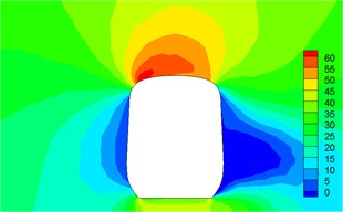
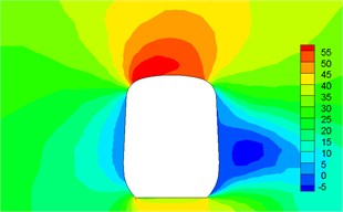
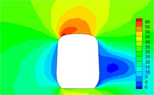
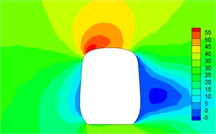
6. Improvement of aerodynamic performance of the high speed train under cross wind
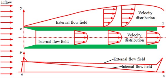
Windbreak devices were usually set along the high speed railway in order to improve running safety of the train under strong cross wind. However, it is equivalent to an auxiliary project of railway and cannot improve own cross wind resistance of the train. Therefore, this paper conducted research from another perspective to study and discuss how to improve own cross wind resistance of the train. At present, the theory of suction and resistance reduction is mainly applied to a flight body. Whether the theory can be applied to reducing aerodynamic loads of the high speed train depended on a negative pressure chamber. Pressure in the chamber was lower than external pressure. Fluids blocked by viscidity on the train surface were pumped away. It was assumed that a straight pipe was in air, and gas flowed around the pipe. Distribution of velocities and pressures inside and outside the straight pipe was shown in Fig. 27.
Fig. 27Distribution of velocities and pressures inside and outside pipe
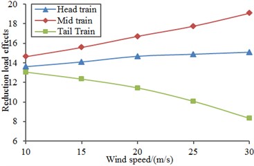
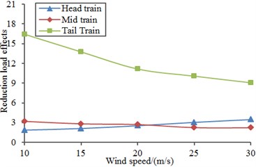
Therefore, this paper considered setting a longitudinal straight pipe in the high-speed train to simulate the suction theory. As for spoiler of the train, airflows flowed through the head train shoulder, generated small separation and then got attached on the train surface once again, where the longitudinal reverse pressure gradient was small. If a longitudinal straight pipe was set on the train and high-speed airflows passed the straight pipe, negative pressures lower than pressures outside the pipe will be generated in the pipe. When the train ran at a high speed, high-speed airflows will flow through in the straight pipe chamber. If the pipe was used to communicate the train surface with the straight chamber, airflows will be sucked into the straight chamber and then flow out from the tail end in the chamber. The straight chamber was a gas suction chamber. However, after the suction chamber was set, pressure in the straight chamber will decrease. In view of effects of crosswind on incoming flows, a certain included angle will be formed between the composited airflow and the longitudinal axis of the straight chamber. Actually, airflows entering the straight chamber will decrease, and the average flow rate of the cross section inside the chamber will decrease. For convenient analysis, it was assumed that the chamber passed the complete train along the longitudinal direction. Train winds generated from high-speed running of the train were directly applied to form high-speed airflows in the chamber, and no fan was needed. If a long chamber in the train was not allowed, where the suction load reduction theory was also feasible, a fan and pipe installed in the train can be used to generate the needed high-speed airflows in the straight chamber, so that a suction function can be achieved. According to the analysis, in view of actual structure of the train body, the suction chamber was set at the position where airflows on the leeward side will get separated, as shown in Fig. 14, where the slot directly communicated with the straight chamber. The slot was 30 mm-40 mm wide; included angle with the horizontal direction was 30°; slot edges were flush with the train surface, as shown in Fig. 28. Aerodynamic performance of the high-speed train with the suction chamber under the cross wind was computed and compared with original results, as shown in Fig. 29. It was shown in the figure that aerodynamic force and force moments of the high-speed train under cross wind will be reduced obviously and running safety of the high-speed train can be improved through application of the suction chamber.
Fig. 28Structure and position of the suction chamber
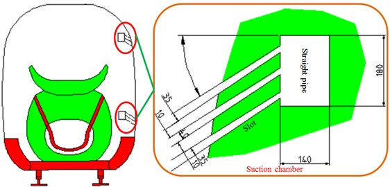
Fig. 29Improvement of aerodynamic performance of the high-speed train under cross wind
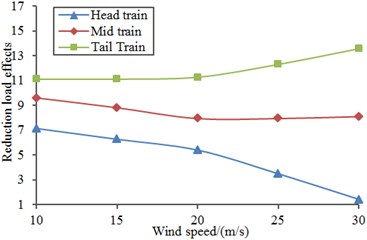
a) Lift
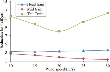
b) Lateral force
c) Overturning moment
d) Shaking moment
7. Conclusions
This paper combined aerodynamics of the high-speed train with system dynamics to study steady and unsteady aerodynamic responses and safety of the high-speed train under cross winds and achieved the following conclusions:
1) Areas of the maximum positive pressures of the high-speed train were partial to the windward side of nose tip of head train; positive pressure areas of tail train were partial to the leeward side of train. Thus, it was clear that head and mid trains bore lateral forces which had the same direction with cross winds while tail train bore lateral force opposite to cross winds.
2) The increase of positive pressures of head and tail trains was mainly affected by train speed. With the increased running speed of train, its positive pressures increased most and negative pressures increased least. Under the same train speed, the positive pressures of head and tail trains increased a lot and negative pressures basically kept unchanged with the increased cross wind speed. Thus, it was clear that train speed was a main factor affecting the size of positive pressures and cross wind velocity had no obvious impacts on the positive and negative pressures of train body.
3) Head train bore the maximum lateral force coefficient, followed by tail train and mid train. Under the same running speed of train, lateral force coefficients of all train bodies increased a lot and presented an approximate linear relationship with the increased cross wind speed. Head train bore the maximum overturning moment coefficient, followed by mid train and tail train. Under the same running speed of train, overturning moment coefficients of all train bodies gradually increased and presented an approximate linear relationship with the increased cross wind speed.
4) There were obvious differences between peak values of power spectral densities of aerodynamic loads of the same high-speed train. The frequency of unsteady aerodynamic loads was within the range of 0 Hz to 25 Hz; main frequency was within the range of 0 Hz to 5 Hz, which was close to the inherent modal frequency of train system. Therefore, the high-speed train was likely to cause the resonance of train bodies and lead to overturn under cross winds.
5) Under cross winds at the speed of 15 m/s, all safety indexes of the high-speed train running at the speed of 250 km/h were within the range of limited values. Derailment coefficient was 0.34; wheel load reduction rate was 0.724; lateral wheel-set force was 34.2 kN; wheel axle vertical force was 88.8 kN. Among them, wheel load reduction rate would exceed limited value most easily.
6) Aerodynamic performance of the high-speed train with the suction chamber under the cross wind was computed and compared with original results. Aerodynamic force and force moments of the high-speed train under cross wind will be reduced obviously and running safety of the high-speed train can be improved through application of the suction chamber.
References
-
Hoppmann U., Koenig S., Tielkes T., et al. A short-term strong wind prediction model for railway application: design and verification. Journal of Wind Engineering and Industrial Aerodynamics, Vol. 90, Issue 10, 2002, p. 1127-1134.
-
Diedrichs B. Studies of Two Aerodynamic Effects on High-Speed Trains: Crosswind Stability and Discomforting Train Body Vibrations Inside Tunnels. KTH, 2006.
-
Khier W., Breuer M., Durst F. Flow structure around trains under side wind conditions: a numerical study. Computers and Fluids, Vol. 29, Issue 2, 2000, p. 179-195.
-
Baker C. J., Jones J., Lopez Calleja F., et al. Measurements of the cross wind forces on trains. Journal of Wind Engineering and Industrial Aerodynamics, Vol. 92, Issue 7, 2004, p. 547-563.
-
Baker C. J. The simulation of unsteady aerodynamic cross wind forces on trains. Journal of Wind Engineering and Industrial Aerodynamics, Vol. 98, Issue 2, 2010, p. 88-99.
-
Suzuki M., Tanemoto K., Maeda T. Aerodynamic characteristics of train/vehicles under cross winds. Journal of Wind Engineering and Industrial Aerodynamics, Vol. 91, Issue 1, 2003, p. 209-218.
-
Diedrichs B., Sima M., Orellano A., et al. Crosswind stability of a high-speed train on a high embankment. Proceedings of the Institution of Mechanical Engineers, Part F: Journal of Rail and Rapid Transit, Vol. 221, Issue 2, 2007, p. 205-225.
-
Ren Z. S., Xu Y. G., Wang L. L., et al. Study on the running safety of high-speed trains under strong cross winds. Tiedao Xuebao, Vol. 28, Issue 6, 2006, p. 46-50.
-
Mao J., Ma X., Xi Y. Research on the running stability of high-speed trains under the cross wind by means of simulation. Journal of Beijing Jiaotong University, Vol. 1, 2011, p. 012.
-
Yu M. G., Zhang J. Y., Zhang W. H. Wind-induced security of high-speed trains on the ground. Journal of Southwest Jiaotong University, Vol. 46, Issue 6, 2011, p. 989-995.
-
Gao G. J. Research on Train Operation Safety under Strong Side Wind. Central South University, Changsha, 2008.
-
Tan S. G., Li X. B., Yang Z., et al. The flow field structure and the aerodynamic performance of high speed trains running on embankment under cross wind. Rolling Stock, Vol. 46, Issue 8, 2008, p. 4-8.
-
Wang Y. G., Chen K. Effects of crosswinds on curve negotiation of high-speed power trains. Journal of Southwest Jiaotong University, Vol. 40, Issue 2, 2005, p. 224-227.
-
Chen K., Luo Y. Effect of the cross wind on the performance of the hydraulic drive power trains on straight line. Rolling Stock, Vol. 41, Issue 6, 2003, p. 22-24.
-
Liu J., Zhang J., Zhang W. Study on characteristics of unsteady aerodynamic loads of a high-speed train under crosswinds by large eddy simulation. Journal of the China Railway Society, Vol. 35, Issue 6, 2013, p. 13-21.
-
Liu J. L., Yu M. G., Zhang J. Y., et al. Study on running safety of high-speed train under crosswind by large eddy simulation. Journal of the China Railway Society, Vol. 33, Issue 4, 2011, p. 13-21.
-
Song Y., Ren Z. S. Research on dynamics performance of high speed trains under strong lateral wind. Rolling Stock, Vol. 44, Issue 10, 2006, p. 4-7.
-
Trainrarini A. Reliability based analysis of the crosswind stability of railway vehicles. Journal of Wind Engineering and Industrial Aerodynamics, Vol. 95, Issue 7, 2007, p. 493-509.
-
Yang Z. G., Ma J., Chen Y., et al. The unsteady aerodynamic characteristics of a high-speed train in different operating conditions under cross wind. Journal of the China Railway Society, Vol. 32, Issue 2, 2010, p. 1-6.
-
Hemida H., Krajnovic S. Numerical study of the unsteady flow structures around train-shaped body subjected to side winds. Proceedings of the European Conference on Computational Fluid Dynamics, Egmond aan Zee, The Netherlands, 2006.
-
Miao X. J., Gao G. J. Aerodynamic performance of train under cross-wind based on DES. Journal of Central South University (Science and Technology), Vol. 7, Issue 43, 2012, p. 2855-2860.
-
Favre T., Efraimsson G. An assessment of detached-eddy simulations of unsteady crosswind aerodynamics of road vehicles. Flow, Turbulence and Combustion, Vol. 87, Issue 1, 2011, p. 133-163.
-
Diedrichs B. Aerodynamic crosswind stability of a regional train model. Proceedings of the Institution of Mechanical Engineers, Part F: Journal of Rail and Rapid Transit, Vol. 224, Issue 6, 2010, p. 580-591.
-
Xiao G. W., Xiao X. B., Wen Z. F. Comparison of dynamic behaviors of wheelsets of high-speed passenger train. Journal of the China Railway Society, Vol. 30, Issue 6, 2008, p. 29-35.
-
Li X. B., Hou C. L., Zhang S. G., et al. Flow-induced vibration of high-speed trains in passing events. Journal of Vibration and Shock, Vol. 28, Issue 4, 2009, p. 81-85.
-
Liu Y. B., Zhang Y. Y., Xing Y. L., Sun Z. X., Yang G. W. Safety analysis of the high speed-train running under the steady aerodynamics forces of cross wind. Science Technology and Engineering, Vol. 14, Issue 8, 2014, p. 76-82.
Cited by
About this article

This work was supported by the National Natural Science Foundation of China (No. 51674121), by the National Natural Science Foundation of Hebei Province (No. E2017209178), Science and Technology Project of Hebei Province (No. 15214104D), the National Natural Science Foundation of Hebei Education Department (No. QN2016088), and Graduate Student Innovation Fund of North China University of Science and Technology, Graduate Student Innovation Fund of Hebei Province (2017S03, CXZZSS2017071).
Ai-min Yang as a professor provided idea and guided this paper, Ce Zhang finished the writing from the beginning to the end, Shanshan Li is responsible for translating this paper, and the other authors checked and submitted this paper to selected journals.
