Abstract
With the continuously increased running speed of high-speed trains, aerodynamic problems become more and more obvious. Running safety of trains under crosswinds is a serious problem among numerous aerodynamic problems. Aiming at this problem, this paper combines computational fluid dynamics with multi-body dynamics to study aerodynamic characteristics and safety problems when the high-speed train is running under crosswinds. Based on fluid software FLUENT, this paper computes the flow field of two high-speed trains passing each other under crosswinds. Meanwhile, with combining the multi-body dynamic software SIMPACK with theories, the paper establishes a multi-body dynamic model of the high-speed train, and applies random aerodynamic loads which act on the high-speed train to this model. Impacts of aerodynamic forces (force moments) on aerodynamic characteristics and running safety of each train compartment in the open air are analyzed. Analyzed results show that: when two high-speed trains are passing each other at the same speed of 350 km/h and the crosswind speed is 15 m/s, maximum pressure fluctuations are at observation points near the lateral windows of the head train; aerodynamic forces and force moments of the head train are more than those of the mid-train and tail-train; the high-speed train still has a high safety performance under crosswinds, where the maximum derailment coefficient is 1.9, the reduction rate of the wheel load is 1.1 and the overturning coefficient is 0.98, all of which are smaller than the limit value. More comprehensive factors are considered by the computational model in this paper. It can be used as an effective method to study and evaluate the performance of two high-speed trains passing each other under crosswinds.
1. Introduction
With the rapid development of high-speed railways, running speeds of high-speed trains are also increased. High-speed trains are developing towards lightweight continuously. The aerodynamic problem caused by the high speed, especially under crosswinds, becomes more and more obvious. Instant pressure waves will be formed when two high-speed trains are passing each other at a high speed, which will lead to horizontal vibrations of trains, damage the window glass of the head train, and seriously influence the running safety and comfort. Therefore, some scholars have conducted the experimental test aiming at this problem. Baker has made a huge contribution to train aerodynamics [1, 2], especially in wind tunnel simulation and test. Through the wind tunnel test, impacts of parameters, speeds and ground features on aerodynamic characteristics under crosswinds were studied [3-5]. Liang [6] used an instant pressure monitoring system to test pressure waves during two high-speed trains passing each other and conducted a comprehensive analysis on tested results. Based on the actual test data of high-speed trains, Liu [7] conducted in-depth analysis on pressure waves of two high-speed trains passing each other in the open air and investigated time-frequency features of pressure waves, as well as relations between main parameters and running speeds. Tian [8] studied the relations between pressure waves of two high-speed trains passing each other and the running speed, train body width, appearance and formation according to the experimental technology of a dynamic model.
These experimental technologies were conducted in field environments or wind tunnels, where the experimental cost was very high, the repeatability was very poor, and only a little of information could be obtained. Numerical simulation is featured by a short research cycle, high speed, lower cost than experimental test, and many difficulties in the experimental test could be overcome. The numerical simulation is only constrained by a few of conditions, so it could acquire more information than the experimental test in general. With quick development of computer technologies and perfection of mesh technologies, numerical models do not require a lot of simplification, and its computational results further approach actual values. Therefore, the numerical simulation technology is widely applied to two high-speed trains passing each other. Kim [9] has proposed a derailing formula of two high-speed trains passing each other under crosswinds, and compared it with traditional derailing formulas and numerical simulation results. Carraini [10, 11] used the line-plane method to compute non-steady aerodynamic forces acting on the train surface, and then conveyed the force to multi-body dynamic software SIMPACK; he also computed running postures of two high-speed trains passing each other and then returned the running postures to fluid software in order to realize coupling between computational fluid dynamics and multi-body dynamics. Tian [12, 13] analyzed pressure waves in two high-speed trains passing each other, studied influential factors of pressure waves by numerical simulation technologies, found the proportional relationship between pressure waves and squares of running speeds, and studied horizontal vibrations of trains. Liu [14] conducted a numerical simulation for aerodynamic characteristics of two high-speed trains passing each other under crosswinds, and found that aerodynamic loads and overturned moments of trains on the leeward side were more than those on the windward side. Ren [15, 16] applied aerodynamic loads of two high-speed trains passing each other under crosswinds to a dynamic model in the form of force elements, conducted a dynamical simulation and obtained safety indexes of the train running under crosswinds. Li [17, 18] studied aerodynamic impacts of two high-speed trains passing each other on lateral windows and obtained a method for evaluating lateral window intensity in the open air. Xi [19] adopted moving grid technologies to conduct a numerical simulation for aerodynamic characteristics of two high-speed trains passing each other, modified the empirical formula and gave a new formula of pressure amplitudes. However, these researches conducted a serious simplification for geometric shapes of trains, or simplified boundary layer models, which cannot reflect the actual situation accurately. The crosswind environment was also neglected in studying aerodynamic characteristics of two high-speed trains passing each other. When the multi-body dynamic model was established, the track spectrum only adopted a vertical irregularity spectrum, but a real track spectrum should include vertical, horizontal and alignment irregularity spectrums. In addition, when pressure waves were computed, aerodynamic loads were simplified into stable loads and applied to the multi-body dynamic model, which was not consistent with the actual situation.
Aiming at shortcomings in these reported researches, this paper studies aerodynamic characteristics of two high-speed trains passing each other under crosswinds. Vertical, horizontal and alignment irregularity spectrums were input into the multi-body dynamic model. Finally, actual random aerodynamic loads were taken as the excitation and applied to the multi-body dynamic model for computing pressure waves of two high-speed trains passing each other under crosswinds. More comprehensive factors are considered by the computational model. It can be used as an effective method to study and evaluate the performance of two high-speed trains passing each other under crosswinds.
2. Mathematical model of two high-speed trains passing each other under crosswinds
2.1. Computational model of aerodynamics
The DES (detached eddy simulation) method based on the Menter - two-equation turbulent flow model was used to solve the Navier-Stokes equation [20-22]. Basic ideas of detached eddy simulation are as follows: a Reynolds time-averaged method is adopted on boundary layers near the wall faces, and small-scale pulsations are simulated by a turbulent flow model; in regions far from the wall face, large eddy simulation is used to simulate detached eddy. The DES equation based on Menter - is as follows:
In the equation, is time, is density, is turbulent kinetic energy, is a directional coordinate, and 1, 2, 3, which are directions in length, width and height in succession; is an airflow velocity component, is a turbulent flow item, , , , , are empirical constants, is a specific dissipation rate of turbulent flow, is a turbulent flow scale parameter; is a switching function which represents the minimum distance between an eddy and the wall face, where in the near wall regions, approaches 1, and the model is approximate to a - model; near the boundary layer edges, approaches 0, and the model is transformed into a - model; is a laminar flow viscosity coefficient, is an eddy viscosity coefficient, and , whereis the absolute value of vorticity, 0.31, the mixed function is as follows:
where: is the minimum distance between the first layer of meshes and the wall face. In the DES method, is substituted by , where is the maximum edge length of elements. The constant is , where the constant item 0.61and 0.78. In this way, on the boundary layer near the wall face, the value is very large, the turbulence kinetic energy value is limited, is far smaller than the mesh scale, the SST turbulent flow model takes effect, and the Reynolds time-averaged method is adopted; at the position far from the wall face, the value is very small, and the changed model acts as a sub-grid Reynolds stress model of large eddy simulation when increases to .
The high-speed train is a thin and long structure. The computational amount will be very large if the numerical simulation is conducted on flow fields of a complete train. With a certain distance away from the head train, flow fields on the train middle part basically have a stable structure. In this paper, a formation model including head train-mid train-tail train was adopted, where the head train and the tail train had the same shape. Meanwhile, in order to avoid excessive meshes, the train was simplified into a geometric body composed of smooth curved faces. Detailed features such as pantographs and bogies were not taken into account. The simplified model of the high-speed train is shown in Fig. 1.
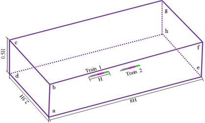
The computational domain of two high-speed trains passing each other under crosswinds is shown in Fig. 2. The train length 78 m was taken as the basis. Therefore, the computational domain was 8.0 H long, 2.5 H wide and 0.5 H high, the distance between two trains was 100 m, the linear distance among two tracks was 5 m, and the distance between the train and the ground was 0.2 m. The left cross section cdhg of the high-speed train was the crosswind inlet boundary and set as the velocity inlet condition, the crosswind velocity was 15 m/s, and the high-speed trains slipped and moved at the constant speed of 350 km/h (slippage mesh method was used to handle the train motion problem, and “interface pair” was used to handle motion parts and stationary parts at the mutual interfaces); other cross sections efgh, aehd and abcd of the high-speed train were the outlet boundaries and set as pressure outlet, where the size was 1 standard atmospheric pressure; the cross section bfgc right above the train was set as a symmetric boundary condition; the train surface was set as a fixed boundary, namely a non-slippage wall face boundary condition; the ground aehd was set as a fixed ground.
Fig. 1Geometric model of the high-speed train
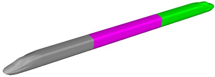
Fig. 2Computational domain of two high-speed trains passing each other
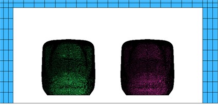
Two opposite running trains were included in the flow field region. Two trains had the same running speeds. In order to solve problems of multi-body region and asymmetry, this paper used a partitioned computation method to divide the computational flow field of two high-speed trains passing each other into 3 parts, as shown in Fig. 3. The observation train, passing train and their nearby flow fields were region 1 and region 2, respectively. These two regions were movable according to expected directions and speeds, respectively. The ground and the flow field far from trains were region 3 which was a fixed part. All parts realized the relative motion by moving contact faces, and real-time data exchange was completed. Different parts had different mesh densities, so movable contact faces among these regions could not be overlaid completely. Therefore, information exchange should be conducted using moving grid technologies when the trains moved forward by one step. When the train moved forward, grids would move together with it, and region 1 and region 2 would be stretched on boundary faces of tail ends to form new grids. Grids were compressed and deleted on front ends. In this way, Shapes of moving contact faces among these regions would be kept unchanged. As a result, different regions of the flow fields could exchange information through moving contact faces. ICEM was used to divide meshes of the computational domain of high-speed trains. Tetrahedral meshes were used to divide the surface. Hexahedral meshes were used to divide fixed parts. Size of three-dimensional meshes was amplified according to a scaling factor. Tetrahedral meshes were adopted for parts far from the train. The maximum size of meshes on the train surface was 80 mm. The maximum size of spatial solid meshes was 1500 mm. The total amount of meshes was about 42.35 million. Surface meshes of the head are shown in Fig. 4. Fig. 5 shows the computational domain meshes of two high-speed trains passing each other.
Fig. 3Requirements for the grid of two high-speed trains passing each other

Fig. 4Surface meshes of the head of high-speed trains
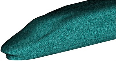
Fig. 5Computational domain meshes of two high-speed trains passing each other

a)
b)
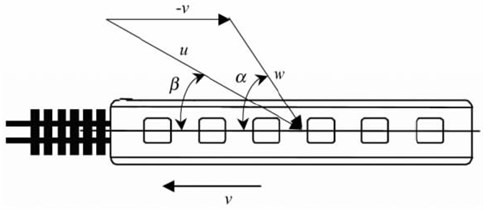
In the model, resultant wind theories were used to simulate the inlet wind velocity, as shown in Fig. 6. The train was deemed to be stationary. Resultant vector was conducted to environmental wind velocity and the reverse velocity – of trains, so the resultant wind velocity was obtained; was a wind direction angle; was a lateral deflection angle. Studied results show that the approximate handling method will not cause obvious errors in general [23-25].
Fig. 6Theories of resultant wind velocity
2.2. Multibody dynamic model of trains
In the model, LM tread was used to match the TB234460 steel track. Based on the equivalent Hertzian contact characteristics, the Fastaim algorithm based on rolling contact non-linear theories was used to compute creep force and creep force moment between wheels and tracks. It is assumed that the displacement vector of the train is as follows:
In the formula, 1; 1, 2; 1, 2, 3, 4; 1, 2, 3, 4, 5, 6, 7, 8. , , and are displacement vectors of train body, framework, wheel-set and axle box, respectively. Letters in the subscript brackets are number of corresponding components. Based on those mentioned hypotheses, the train-track coupling dynamic equation could be established, as follows:
In the formula, is a mass matrix; is a damping matrix; is a rigidity matrix; and Fav are equivalent forces caused by track irregularity and aerodynamic loads under crosswinds. It is found that Eq. (5) has considered aerodynamic effects of the train, the track irregularity is an important factor which leads to train vibration and affects running safety performance. In this paper, the irregularity spectrum was taken as the track excitation. Aerodynamic loads borne by the train which ran under the crosswind environment were loaded into the dynamic model. The dynamic Eq. (5) was solved. In this way, dynamic characteristics of the high-speed train which ran under crosswinds could be obtained.
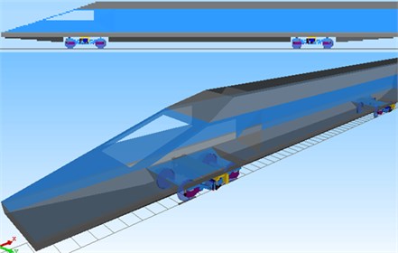
In this paper, SIMPACK software was used to establish a multi-body dynamic model of the high-speed train. The dynamic model was composed of 15 components including 1 train body, 4 wheel-sets, 2 frameworks and 8 rotational arms. The rigid train body, frameworks and wheel-sets had 6 degrees of freedom, namely vertical direction, longitudinal direction, horizontal direction, head shaking, nodding and lateral rolling; rotational arms had 1 degree of freedom, namely nodding; the dynamic model of each train had 50 degrees of freedom, and the dynamic model of the complete train had 150 degrees of freedom. Structures of each system were represented by equivalent spring, damping and mass blocks; the track system adopted a dual-mass (sleeper and track bed) three-layer (steel track, sleeper, track bed and road bed) track model with spring-damping vibration continuous distribution. The dynamic model of a train established by the multi-body dynamic software SIMPACK is shown in Fig. 7. Each component was deemed as a rigid body.
Fig. 7Multi-body dynamic model of the high-speed train
Modern steel tracks are not an ideal flat and straight state, where the real track spectrum should include vertical, horizontal and alignment irregularity spectrums. Due to these spectrums, interactions are caused between wheels and tracks, and geometric shapes of tracks will be changed, so that the tracks are randomly unbalanced. The stability of high-speed trains will be reduced. Therefore, this paper input vertical, horizontal and alignment irregularity spectrums to the multi-body dynamic model, as shown in Fig. 8. It is also shown in this figure that the amplitude difference of track spectrums in three directions was not large, so any track spectrum cannot be neglected. Therefore, the actual engineering should use the irregularity spectrum in three directions as the excitation.
Fig. 8Irregularity spectrums in three directions of high-speed trains
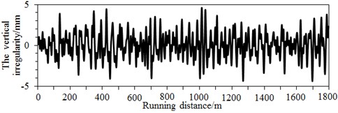
a) Vertical irregularity spectrum

b) Horizontal irregularity spectrum

c) Alignment irregularity spectrum
3. Flow fields of two high-speed trains passing each other under crosswinds
Pressure distributions on surfaces of the leeward train and the windward train during two high-speed trains passing each other on the flat ground at the same speed of 350 km/h, when the crosswind velocity is 15 m/s and the wind direction angle is 90°, as shown in Fig. 9. At the moment 0.255 s, two trains did not meet yet; due to the crosswind, the maximum positive pressure region of two trains leant to the windward side; large negative pressure regions were on the leeward side of two trains; a part of positive pressure regions were also at the tail part. At the moment 0.51s, heads of the leeward train and windward train were meeting, and pressure regions on heads of two trains would interact; due to two trains passing each other, airflows among two trains would get extruded, so the negative pressure region on the windward side would be weakened, and the negative pressure region of the leeward train became larger. At the moment 0.765 s, heads of the leeward train and windward train just met mid-trains of another train, where positive pressures were distributed on heads, positive pressures on the windward side were decreased, while negative pressures on the leeward side were increased. At the moment 1.02 s, tail trains of the leeward train and windward train just met mid-trains of another trains, where head regions of two trains were positive pressures, and most of the leeward side was negative pressures. At the moment 1.275 s, tail trains of the leeward train and windward train just met, where positive pressures in tail regions of two trains were increased, pressures on the windward side of the windward train were positive, while the leeward side was the negative pressure region; negative pressures were distributed on two sides of the leeward train. When the moment passed 1.53 s, pressure distributions of the leeward train and windward train were recovered, where the changes were not obvious.
Fig. 9Pressure contours of two high-speed trains passing each other under crosswinds

a) Moment 0.255 s

b) Moment 0.510 s

c) Moment 0.765 s

d) Moment 1.020 s

e) Moment 1.275 s

f) Moment 1.530 s

g) Moment 1.785 s
Fig. 10 shows contours of surface pressures at 0.765 s and 1.02 s when two high-speed trains are passing each other under crosswinds. The reasons for choosing the moments 0.765 s and 1.02 s for flow field analysis are that there are obvious eddies on the side of the train, and they have a good representation. Fig. 11 shows contours of surface pressures at 0.765 s and 1.02 s when two high-speed trains are passing each other under the working condition without crosswinds. It is found through comparison between Fig. 10 and Fig. 11 that when the high-speed train met at the same speed under crosswinds, positive pressures on the leeward side of head trains were increased, where the positive pressure region of the head train of leeward train was more than that of the windward train. Meanwhile, two large eddies with different rotation directions were on the leeward side of the leeward train. Eddies were small on the leeward side of the windward train. Due to these eddies, the instability of the train was further intensified, so that trains bore a large pressure difference. Under the working condition without crosswinds, two large eddies were also on the side without meeting, where no eddy was on the side with two high-speed trains passing each other. Under the working condition with crosswinds, two eddies with different rotation directions and sizes were on the side with two high-speed trains passing each other. It is thus clear that during two high-speed trains passing each other, the derailment of the leeward train will be caused more easily due to crosswinds, so that it had the poorest safety performance. Therefore, the paper will make a detailed analysis on pressure fluctuations on the leeward train and analyze its safety performance.
Fig. 10Pressure distributions on the cross section with crosswinds
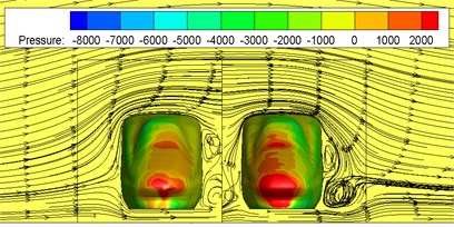
a) Moment 0.765 s
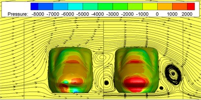
b) Moment 1.020 s
Fig. 11Pressure distributions on the cross section without crosswinds
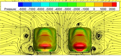
a) Moment 0.765 s
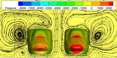
b) Moment 1.020 s
Fig. 12 shows surface pressures of the windward train and leeward train during meeting of nose tip of two trains. It is shown in Fig. 12 that compared with the meeting without crosswinds in Fig. 13, when two high-speed trains were passing each other under crosswinds, the pressure distribution on surfaces presented both the crosswind and meeting characteristics.
Fig. 12Contours of surface pressures of trains with crosswinds
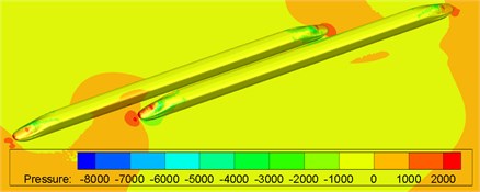
a) Moment 0.765 s
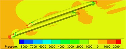
b) Moment 1.020 s
Fig. 13Contours of surface pressures of trains without crosswinds
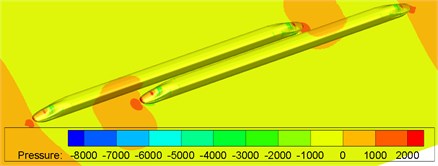
a) Moment 0.765 s
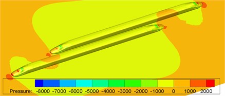
Moment 1.020 s
4. Pressures of two high-speed trains passing each other under crosswinds
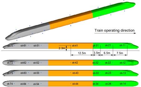
During two high-speed trains passing each other under crosswinds, the aerodynamic impacts borne by the leeward train were more serious than those of the windward train. Therefore, the paper mainly takes the leeward train as the studied object. In order to learn about relations of surface pressure waves during two high-speed trains passing each other under crosswinds, measure points were selected on the head train, mid-train and tail train of the leeward train, as shown in Fig. 14. The distance between the measure point on the mid-train and the windshield was 12.5 m; distances between the measure points of the head and the windshield were 3.5 m, 10 m and 17.5 m, respectively; measure points on surfaces of the windward side and leeward side were 2.3 m high above the ground; corresponding measure points on the train top and bottom were arranged at the middle positions of the longitudinal center face. Numbers of these measure points were named as follows: ot-11, ot-21, ot-31, ot-41, ot-51, ot-61 and ot-71 were measure points on the surfaces near the wall face (windward side); ot-12, ot-22, ot-32, ot-42, ot-52, ot-62 and ot-72 were measure points on middle surfaces of the top; ot-13, ot-23, ot-33, ot-43, ot-53, ot-63 and ot-73 were measure points on surfaces far from the wall face (leeward side); ot-14, ot-24, ot-34, ot-44, ot-54, ot-64 and ot-74 were measure points on the middle surfaces of the bottom. Detailed positions of measure points are shown in Fig. 14.
Fig. 14Schematic diagram of pressure measure points on surfaces
4.1. Pressure waves of two high-speed trains passing each other under crosswinds
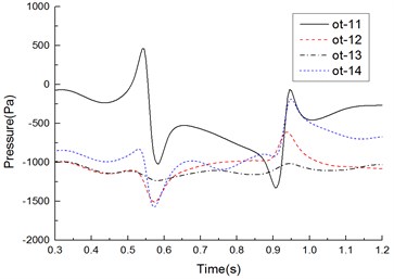
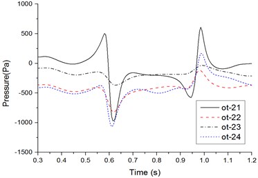
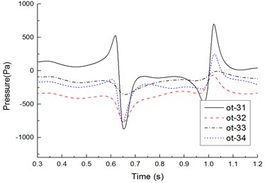
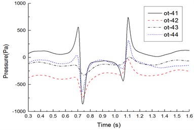
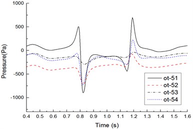
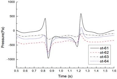
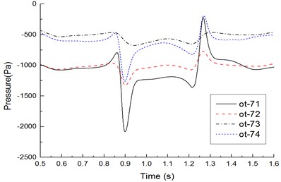
Fig. 15 shows time-history curves of each measure point during two high-speed trains passing each other. Table 1 shows compared results of peak values of measure points. Analyzed results from Fig. 15 and Table 1 show that:
1) Before the head of the windward train reached measure points on the lateral window of the leeward train, pressures already started increasing. Then, pressures were increased quickly. When the nose tip of the windward train reached the measure point, a positive pulse and a negative pulse were caused, namely the head wave. After the maximum negative pulse was caused, fluctuations with constant amplitudes would be started till the nose tip of the tail train of the windward train passed the measure point when a negative pulse and a positive pulse were generated, namely a tail wave.
2) During two high-speed trains passing each other, the head wave of the pressure full wave was more than the tail wave; absolute values of the negative wave were more than those of the positive wave, which was more obvious in the tail train.
3) On the cross section, peak values of each measure point were characterized in that: peak value distribution of the head wave was 11 > 14 > 13 > 12; peak value distribution of the tail wave was 11 > 14 > 13 > 12 (other measure points on the cross section had the same distribution); obviously, pressure peak values changed more obviously on the train meeting side (namely windward side), the train bottom position ranked the second place, the non-train meeting side (namely leeward side) ranked the third place, and the train top position ranked the last.
4) Along the running direction, head wave and tail wave peak values of measure points in the same longitudinal direction were decreased, where the measure point ot-11 (near the lateral window) had the maximum peak value; the head wave peak value was 1486 Pa; the tail wave peak value was 1279 Pa, as shown in Table 1.
5) During two high-speed trains passing each other, the pressure region on the meeting side was more than that on another side; negative pressures with large-area appeared on the non-train meeting side, train top and bottom; fewer positive pressure regions appeared on the meeting side compared with another side. Obviously, breaking of the lateral window glass during two high-speed trains passing each other is caused by that the window glass would be sucked out by the meeting negative pressures, where the breaking is not caused by positive pressure impacts.
6) Positive wave amplitudes of head waves on the windward side were positive pressures, and negative wave amplitudes of head waves were negative pressures; during two high-speed trains passing each other under crosswinds, positive wave and negative wave amplitudes of head waves on measure points of the top, non-train meeting side and bottom were negative pressures. Therefore, the high-speed train had the large lateral force and head shaking force moment.
7) Positive wave amplitudes of tail waves on each measure point were negative pressures (except for measure points on the windward side), and negative wave amplitudes of tail waves were negative pressures; in tail waves, the measure point on the windward side had the largest pressure peak value 1279 Pa, the pressure peak value on the measure point of the bottom ranked the second place, the peak value of measure points on the non-train meeting side ranked the third place, and the measure point on the top had the minimum pressure peak value. It is thus clear that the head train and tail train were affected by crosswinds seriously, and they had the poorest running safety performance under crosswinds.
Table 1Comparison of peak values of each measure point
Measure points | ||||||
ot-11 | 469 | –1017 | 1486 | –53 | –1332 | 1279 |
ot-21 | 508 | –968 | 1476 | 604 | –576 | 1180 |
ot-31 | 529 | –872 | 1401 | 702 | –492 | 1194 |
ot-41 | 564 | –860 | 1424 | 744 | –439 | 1183 |
ot-51 | 507 | –895 | 1402 | 698 | –442 | 1140 |
ot-61 | 434 | –960 | 1394 | 601 | –558 | 1159 |
ot-71 | –786 | –2089 | 1303 | –220 | –1362 | 1142 |
ot-12 | –1095 | –1512 | 417 | –188 | –970 | 782 |
ot-22 | –405 | –827 | 422 | –118 | –422 | 304 |
ot-32 | –380 | –767 | 387 | –65 | –334 | 269 |
ot-42 | –359 | –740 | 381 | –24 | –327 | 303 |
ot-52 | –362 | –709 | 347 | –73 | –342 | 269 |
ot-62 | –395 | –734 | 339 | –144 | –417 | 273 |
ot-72 | –966 | –1322 | 356 | –772 | –1077 | 305 |
ot-13 | –1119 | –1239 | 120 | –1017 | –1151 | 134 |
ot-23 | –143 | –367 | 224 | –32 | –180 | 148 |
ot-33 | –147 | –369 | 222 | –8 | –146 | 138 |
ot-43 | –136 | –327 | 191 | 6 | –134 | 140 |
ot-53 | –123 | –293 | 170 | –34 | –153 | 119 |
ot-63 | –143 | –302 | 159 | –93 | –217 | 124 |
ot-73 | –460 | –674 | 214 | –467 | –655 | 188 |
ot-14 | –826 | –1572 | 746 | –183 | –919 | 736 |
ot-24 | –369 | –1067 | 698 | 169 | –438 | 607 |
ot-34 | –126 | –763 | 637 | 252 | –274 | 526 |
ot-44 | 40 | –624 | 664 | 312 | –205 | 517 |
ot-54 | –56 | –733 | 677 | 231 | –299 | 530 |
ot-64 | –144 | –821 | 677 | 118 | –428 | 546 |
ot-74 | –482 | –1263 | 781 | –197 | –820 | 623 |
4.2. Aerodynamic forces (force moment) of two high-speed trains passing each other under crosswinds
After the flow field of high speed trains was computed, aerodynamic loads which acted on the high-speed train under crosswinds should be loaded into the multi-body dynamic model, and running safety of the high-speed train can be analyzed. According to force translation and equivalence principles, distributed pressures acting on the train surface were simplified to a point of the train. Therefore, concentrated force and force moment acting on this point were obtained. Through simplification, resistance, lateral force, lift force, overturning force moment, head shaking force moment and nodding force moment acting on each train under different wind direction angles, different wind velocities and different running speeds could be obtained. In those reported researches, aerodynamic forces were basically simplified into stable loads. For example, Liu [26, 27] has applied stable aerodynamic loads to the multi-body dynamic model.
Fig. 15Time-history curves of each measure point on cross sections
a) Measure points on cross section 1
b) Measure points on cross section 2
c) Measure points on cross section 3
d) Measure points on cross section 4
e) Measure points on cross section 5
f) Measure points on cross section 6
g) Measure points on cross section 7
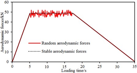
However, using the stable load as the excitation and applying it to the multi-body dynamic model cannot satisfy actual situations. Therefore, in this paper, random aerodynamic loads were applied to the high-speed train, as shown in Fig. 16. During 0-5 s, the aerodynamic force was loaded linearly, so running of the high-speed train gradually tended to be stable. Aerodynamic forces acted within 5-18 s. Then, the force reached 0 through linear unloading.
Fig. 16Two different kinds of loading methods
Computational coordinates of aerodynamic forces and force moment during two high-speed trains passing each other are shown in Fig. 17, where the axis is the resistance direction; axis is the lift force direction; axis is the lateral force direction; lateral rolling force moment was rotated around the axis; head shaking force moment was rotated around the axis; nodding force moment was rotated around axis. Simplified centers of aerodynamic forces and aerodynamic force moments in this paper are shown in Fig. 17, where the center was 2.1 m high above the ground; the center of the head train was 12.5 m away from the windshield; the center of the mid-train was also 12.5 m away from the windshield; the center of the tail train was 12.5 m away from the windshield; the force moment center was arranged on the center face in the longitudinal direction.
Fig. 17Schematic diagram of the aerodynamic force and moment
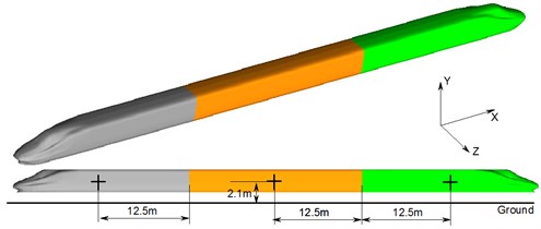
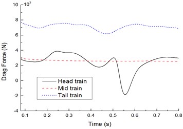
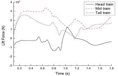
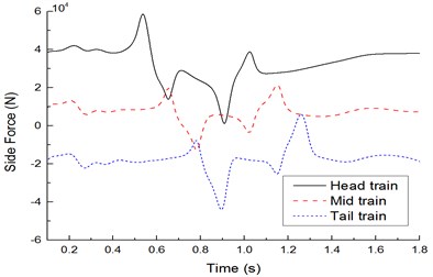
Fig. 18 shows change curves of resistance, lift force and lateral force on the leeward train during two high-speed trains passing each other under crosswinds. It is shown in Fig. 18 that: (1) Resistance characteristics: During two high-speed trains passing each other, resistance changed violently on the head train due to crosswinds, opposite resistance was borne during tail train meeting, resistance of the mid-train did not change obviously throughout the train meeting, and the tail train bore the maximum resistance with the amplitude 7000 N. (2) Lift force characteristics: During two high-speed trains passing each other under crosswinds, lift forces of the head train changed violently, where it bore the downward lift force before two high-speed trains passing each other and bore upward lift force during tail train meeting; both the mid-train and the tail train bore the upward lift force. (3) Lateral force characteristics: Lateral force values caused by the head train and tail train had the largest effects, and the lateral force peak of head waves in the head train was more than that of tail waves; when the windward train head passed the leeward train, a positive lateral force peak was caused by the head train, mid-train and tail train of the leeward train firstly, and then the lateral force was sharply decreased to a negative peak value; when the windward train tail passed the head train of the leeward train, the leeward train generated a negative peak value at first, and then the lateral force was increased to a positive peak value sharply.
Fig. 18Time-history curves of aerodynamic forces of each train body
a) Comparison of resistance
b) Comparison of lift forces
c) Comparison of lateral forces
Fig. 19 shows time-history curves of lateral rolling force moments on the leeward train during two high-speed trains passing each other under crosswinds. It is shown in Fig. 19 that: When the head or tail parts of the windward train passed the leeward train, the lateral rolling force moment of the leeward train had 3 peaks. The head train of the leeward train generated a negative peak at first. Next, when the windward train head passed 1/4 train length, the lateral rolling force moment was increased to the peak sharply and then experienced a negative peak with the opposite direction. When the windward train tail passed the head train of the leeward train, the leeward train generated a peak value of upward lateral rolling force moment at first; then, the lateral rolling force moment was decreased to a negative peak sharply; next, the lateral rolling force moment was increased to a positive peak sharply. Lateral rolling force moments of the complete train experienced 6 direction changes.
Fig. 19Time-history curves of lateral rolling force moments of each train body
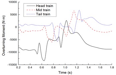
Obviously, during two high-speed trains passing each other, each train body experienced 6 impact force moments with outward, inward, outward, inward, outward and inward directions. During two high-speed trains passing each other, the head train had the largest lateral rolling force moment amplitude; the tail train ranked the second place; the mid-train ranked the last. Therefore, in the subsequent dynamic analysis, only the safety performance of the head train was analyzed.
4.3. Running safety of two high-speed trains passing each other under crosswinds
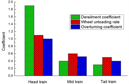
According to Reference [28, 29], dynamic evaluation indexes of the train include derailment coefficient, reduction rate of wheel load and overturning coefficient. Derailment coefficient refers to the ratio of horizontal forces to vertical forces acting on wheels at a moment, where the evaluation limit value of the derailment coefficient is 2.0; the reduction rate of wheel loads is defined as , where is the reduction number of wheels on one side, and is average wheel loads on left and right sides. The limit value 1.2; while a train is running along a rail, the train would bear various types of horizontal forces including wind forces, centrifugal forces, gravity and horizontal inertia forces. Under impacts of these forces, the train may overturn. The limit value of overturning coefficient is 1.0.
Fig. 20 shows a comparison of derailment coefficient, reduction rate of wheel loads and overturning coefficient of each train body under the working conditions: crosswind velocity is 15 m/s and running speed is 350 km/h. It is shown in Fig. 20 that the head train was the most unsafe, where the derailment coefficient was 1.9, the reduction rate of wheel loads was 1.1 and the overturning coefficient was 0.98, all of which were smaller than the limit value. Therefore, the high-speed train still had a high safety performance under the working conditions.
Fig. 20Analysis on running safety of each train body
5. Conclusions
The paper conducted a numerical simulation for two high-speed trains passing each other using the moving grid technology, where vertical, horizontal and alignment irregularity spectrums were input into the multi-body dynamic model. The actual random aerodynamic loads were taken as excitation and applied to the multi-body dynamic model for computing pressure waves of two high-speed trains passing each other. More comprehensive factors were considered by this computational model. It can be used as an effective method to study and evaluate the performance of two high-speed trains passing each other under crosswinds. Affected by crosswinds, the nose tip of the head train is not a pressure stagnation point any longer. The maximum pressure tends to the windward side of the head train, so that the head train is the most unsafe. Therefore, materials of this part should have higher pressure resistance than other parts. At earlier stage of two high-speed trains passing each other, trains will bear an outward repulsive force; at middle stage, trains will bear an inward suction force; at later stage, trains will bear an outward repulsive force again. Changing features of the lateral force in two high-speed trains passing each other will affect their running safety seriously. Therefore, it is feasible to design some pumping-suction chambers on trains in order to change the inward suction force during two high-speed trains passing each other. This paper only studied aerodynamic characteristics of two high-speed trains passing each other on a linear track, but failed to deal with this problem on a curved line track. Safety problems of two high-speed trains passing each other on a curved line track still require in-depth discussion. In addition, with development of high-speed trains, this simulation model should be modified continuously to match the latest trains. In this way, more accurate results could be obtained. All the work will be studied in the future.
References
-
Baker C. J., Quinn A., Sima M., et al. Full-scale measurement and analysis of train slipstreams and wakes. Part 1: Ensemble averages. Proceedings of the Institution of Mechanical Engineers, Part F: Journal of Rail and Rapid Transit, Vol. 228, Issue 5, 2014, p. 451-467.
-
Cui K., Yang W., Gou H. Experimental research and finite element analysis on the dynamic characteristics of concrete steel bridges with multi-cracks. Journal of Vibroengineering, Vol. 19, Issue 6, 2017, p. 4198-4209.
-
Bell J. R., Burton D., Thompson M., et al. Wind tunnel analysis of the slipstream and wake of a high-speed train. Journal of Wind Engineering and Industrial Aerodynamics, Vol. 134, 2014, p. 122-138.
-
Morden J. A., Hemida H., Baker C. J. Comparison of RANS and detached eddy simulation results to wind-tunnel data for the surface pressures upon a class 43 high-speed train. Journal of Fluids Engineering, Vol. 137, Issue 4, 2015, p. 041108.
-
Li J. Q., He S. Q., Ming Z. An intelligent wireless sensor networks system with multiple serves communication. International Journal of Distributed Sensor Networks, Vol. 7, 2015, p. 1-9.
-
Liang X. F., Tian H. Q. Test research on crossing air pressure pulse of 200km/h eletric multiple unit. Journal of Central South University of Technology, Vol. 33, Issue 6, 2002, p. 621-624.
-
Liu L., Gao P. X. Characteristic analysis of air pressure wave generated by high-speed train passing each other. China Measurement and Test, Vol. 42, Issue 7, 2016, p. 93-96.
-
Tian H. Q. Research and applications of air pressure pulse from trains passing each other. Journal of Railway Science and Engineering, Vol. 1, Issue 1, 2004, p. 83-89.
-
Kim M. S., Kim G. Y., Kim H. T., et al. Theoretical cross-wind speed against rail vehicle derailment considering the cross-running wind of trains and the dynamic wheel-rail effects. Journal of Mechanical Science and Technology, Vol. 30, Issue 8, 2016, p. 3487-3498.
-
Carrarini A. Coupled Multibody-aerodynamic simulation of high-speed trains manoeuvres. PAMM, Vol. 2, Issue 1, 2003, p. 114-115.
-
Carrarini A. Reliability based analysis of the crosswind stability of railway vehicles. Journal of Wind Engineering and Industrial Aerodynamics, Vol. 95, Issue 7, 2007, p. 493-509.
-
Tian H. Q., Xu P., Liang X. F., Liu T. H. Correlation between pressure wave of train passing and running speed. China Railway Science, Vol. 27, Issue 6, 2006, p. 64-67.
-
Tian H. Q., He D. X. 3-D numerical calculation of the air pressure pulse from two trains passing by each other. Journal of the China Railway Society, Vol. 23, Issue 3, 2001, p. 18-22.
-
Liu F., Yao S., Zhang J., Zhang N. Aerodynamic effect of EMU passing by each other under crosswind. Journal of Central South University (Science and Technology), Vol. 47, Issue 1, 2016, p. 307-313.
-
Ren Z. S., Xu Y. G., Wang L. L., Qiu Y. Z. Study on the running safety of high-speed trains under strong cross winds. Journal of the China Railway Society, Vol. 28, Issue 6, 2006, p. 46-50.
-
Ren Z. S., Liu Z. M. Vibration and frequency domain characteristics of high speed EMU. Journal of Mechanical Engineering, Vol. 49, Issue 16, 2013, p. 2-7.
-
Li R. X., Zhao J., Liu J., Zhang W. H. Influence of air pressure pulse on side windows of high-speed trains passing each other. Journal of Mechanical Engineering, Vol. 46, Issue 4, 2010, p. 87-98.
-
Li R. X., Liu J., Qi Z. D., Zhang W. H. Air pressure pulse developing regularity of high-speed trains crossing in open air. Journal of Mechanical Engineering, Vol. 47, Issue 4, 2011, p. 125-130.
-
Xi Y. H., Mao J., Liu R. D., Yang G. W. A probe into air pressure pulse amplitude of high-speed trains corssing in open air. Journal of South China University of Technology (Natural Science Edition), Vol. 44, Issue 3, 2016, p. 118-127.
-
Cui K., Zhao T. T. Unsaturated dynamic constitutive model under cyclic loading. Cluster Computing, 2017, p. 1-11, https://doi.org/10.1007/s10586-017-0881-9.
-
Wei W., Fan X., Song H., et al. Imperfect information dynamic stackelberg game based resource allocation using hidden Markov for cloud computing. IEEE Transactions on Services Computing, 2016, p. 1-13.
-
Yang A., Han Y., Pan Y., et al. Optimum surface roughness prediction for titanium alloy by adopting response surface methodology. Results in Physics, Vol. 7, 2017, p. 1046-1050.
-
Cui K., Qin X. Virtual reality research of the dynamic characteristics of soft soil under metro vibration loads based on BP neural networks. Neural Computing and Applications, 2017, p. 1-10, https://doi.org/10.1007/s00521-017-2853-7.
-
Wei W., Song H., Li W., et al. Gradient-driven parking navigation using a continuous information potential field based on wireless sensor network. Information Sciences, Vol. 408, 2017, p. 100-114.
-
Yang K., Yang N., Xing C. W., et al. Space-time network coding with transmit antenna selection and maximal-ratio combining. IEEE Transactions on Wireless Communications, Vol. 14, Issue 4, 2015, p. 2106-2117.
-
Liu Y. B., Zhang Y. Y., Xing Y. L., Sun Z. X., Yang G. W. Safety analysis of the high speed-train running under the steady aerodynamics forces of cross wind. Science Technology and Engineering, Vol. 14, Issue 8, 2014, p. 76-82.
-
Li J., Yu F. R., Deng G., et al. Industrial internet: a survey on the enabling technologies, applications, and challenges. IEEE Communications Surveys and Tutorials, 2017, p. 1-1.
-
Xiang C. Q., Guo W. H., Zhang J. W. Overturning stability of a high-speed train running on a bridge and optimal height of wind barriers under strong crosswind. Journal of Vibration and Shock, Vol. 33, Issue 12, 2014, p. 80-86.
-
Ge C., Sun Z. L., Wang N., et al. Energy management in cross-domain content delivery networks: a theoretical perspective. IEEE Transactions on Network and Service Management, Vol. 11, Issue 3, 2014, p. 264-277.
