Research on the distribution of aerodynamic noises of high-speed trains

1. Introduction

With the constant development of high-speed trains, the noise problem of high-speed trains becomes increasingly prominent. As a comfort index which can be directly perceived by drivers and conductors, noises have gradually turned into a key factor affecting the business operation of high-speed trains [1]. At a high speed, the dynamic environment of train operation is mainly aerodynamic action [2]. When the train speed exceeds 300 km/h or wheel-rail noises are treated, aerodynamic noises will replace wheel-rail noises and become the main sound source of high-speed trains [3]. Aerodynamic noises caused by the operation of high-speed trains become the factor of restricting the speed. Regarding Japanese S250 high-speed trains, their design speed and experimental speed are more than 350 km/h, but their aerodynamic noises reach an unbearable level. Finally, these kinds of trains have to run at the speed of 300 km/h. Similarly, the design speed of maglev trains is over 430 km/h. Limited by noise criteria, trains have to run at the speed of 200 km/h [4-6].

High-speed trains make constant development through introduction, absorption and re-innovation. Compared with research on structures and system, researches on aerodynamic noises are relatively backward. At present, the aerodynamic noise of high-speed trains is studied mostly through numerical computation. Due to the complexity of the problem, most of computations lay emphasis on aerodynamic noises at a certain part of high-speed trains. Xiao [7] took the longitudinal symmetrical plane of high-speed train as the researched object, established a large eddy simulation model for the longitudinal symmetrical plane of high-speed trains, studied the spectral characteristics and change rule of aerodynamic noises in the longitudinal symmetrical plane and obtained the optimal shape of junction. Liu [8] established a mathematical model for the three-dimensional flow field of head train of high-speed trains, used Lighthill acoustic analogy theory to compute the aerodynamic noise of high-speed trains in the far field, and applied a broadband noise source model to compute aerodynamic noises at the surface of high-speed trains. Zhang [9] adopted detached eddy simulation (DES) and Lighthill acoustic analogy theory to study different structures and installation positions, and obtained the layout proposal of pantograph that the sound pressure level of the whole train reduced by 3.2 dBA at most. Yan [10] built a computational model including head train, middle train and tail train and computed noise source intensity and far-field noises at the surface of body. The model did not consider bogies or make a specific analysis and summary for noise results in the far field. Yuan [11] established a computational model including head train and tail train, computed aerodynamic noise source intensity and aerodynamic noise at the surface of body and improved computational accuracy compared with the model only established for the head train. Zhang [12] built an aerodynamic model including head train, middle train and tail train, computed the near-field and far-field aerodynamic noise of high-speed trains and only took into account noise sources at the surface of body instead of bogies and pantograph. Sun [13] established the aerodynamic model of 3-train formation, conducted an analysis on the flow field characteristics of train head, junction and tail, and studied the contribution of different parts of body to aerodynamic noises. Bogies and pantograph were not considered in the model. Liu [14] used Green function of half-free space to solve FW-H equation according to the actual situation of high-speed trains, established an acoustic integral formula considering ground effect, studied the impact of ground effect on the aerodynamic noise of high-speed trains, and made the computation of noises under trains more accurate. Yang [15] numerically simulated and analyzed external flow field and aerodynamic noises with and without air deflector and pointed out that reasonable design could enable the air deflector to well guide airflow so as to reduce aerodynamic noises in the power collection equipment. Du [16] adopted separated vortex turbulence model and acoustic analogy theory to predict the aerodynamic noise of simplified pantograph. Results showed that beams at the top of pantograph were main sources of aerodynamic noises. Yu [17] adopted nonlinear acoustic solver and acoustic analogy theory to carry out numerical research on 3 kinds of pantograph air deflectors and found their sound pressure level decreased by 3 dB in the case of designing the air deflector structure of pantograph similar to windshield in a span-wise direction. Huang [18] established an analytical model for the aerodynamic noise of bogies, focused on studying aerodynamic noises when bogies were noise sources, and analyzed the noise reduction effect of bogies on both sides of radiation noises in the case of applying the apron board of bogies. References [19] carried out numerical research on the aerodynamic noise of trailer bogies and obtained the far-field aerodynamic noise of trailer bogies which was broadband noise with directivity, attenuating characteristics, amplitude characteristics and so on.

Currently, a lot of studies have been conducted on the aerodynamic noise of high-speed trains. However, the computation of overall aerodynamic noise of high-speed trains only considers the surface of body in general due to the complexity of problem. Namely, only the structure surface of body is taken as aerodynamic noise source and pantograph and bogie [20-22] as main aerodynamic noise sources of high-speed trains are neglected. The difficult point of the problem is that pantograph and bogie have complex structures and their dimensions are relatively small compared with that of body. It is thus difficult to establish the computational model of aerodynamics including body, pantograph and bogie. This paper adopted a modular modeling method, firstly built the overall aerodynamic model of body of high-speed trains, built pantograph and bogie models separately, assembled bogies and pantograph into the corresponding positions of body, established a computational mode for the aerodynamic noise of the whole train composed of head train, middle train, tail train, 6 bogies, 3 air conditioning, 1 pantograph area and 1 pantograph, and obtained the aerodynamic flow behavior of high-speed train, the distribution of aerodynamic noises of trains, the propagation characteristics of pantograph aerodynamic noises and so on.

2. Analytical theories of aerodynamic noises of high-speed trains

Aerodynamic noises are the result of interaction between fluid and structure when fluid flows through solid surface. As general fluid computation software, Fluent integrates strong computing capacity of aerodynamic noises. Fluent can directly obtain the generation and propagation of sound wave through solving fluid dynamic equations. The direct simulation method is called as CAA (Computational Aero Acoustics) which accurately simulates viscosity effect and turbulence effect through directly solving unsteady N-S equation and unsteady Reynolds average RANS equation [23, 24]. CAA method calls for high-precision numerical solution method, fine meshes and nonreflecting boundary conditions of sound wave. Therefore, computational cost is high. Currently, this method cannot be adopted to solve the aerodynamic noise problem of high-speed trains. Another computational method in Fluent is widely used Lighthill acoustic analogy method, also known as AAA (Aero-Acoustic Analogy) method. Different from CAA method, “noise analogy” method decouples wave equation and flow equation, first solves unsteady flow equations, then takes the solution result as the noise source and separates sound wave solution from flow solution through solving wave equation and obtaining acoustic wave solution, which improves computational efficiency and makes solving large and complex pneumatic acoustic problems possible. Based on the mass and momentum conservation equation of fluid mechanics, Lighthill [25] deduced the wave equation of aerodynamic noises generated by turbulence within the scope of small scales surrounded by static fluid as follows:

wherein, $\rho \text{'}$ was the disturbance quantity of fluid density, $\rho \text{'}=\rho -{\rho }_o$. $\rho$ and ${\rho }_o$ represented density in a disturbed and undisturbed state respectively. $T_{ij}$ was Lighthill stress, $T_{ij}=\rho u_i{u}_j-e_{ij}+{\delta }_{ij}(p-c_0^2\rho )$. $e_{ij}$ stood for viscous stress. ${\delta }_{ij}$ was Kronecker delta. $c_o$ was sound velocity. The left end of Eq. (1) was the same with general acoustic equations. The right end of Eq. (1) was equivalent to sound source item and called as Lighthill sound source item. If the right end item was 0, the equation transformed into general acoustic wave equation with sound velocity $c_0$ in static fluid. As a matter of fact, the right end of Eq. (1) contained variable $\rho$. Therefore, Eq. (1) was not acoustic wave equation in a real sense. In essence, Eq. (1) was still fluid flow equation. However, Lighthill pointed out that Eq. (1) was a typical acoustic wave equation if the right end of the equation was regarded as a quadrupole source item. As a result, the method was called as “noise analogy” method.

Lighthill equation was taken as the foundation. FW-H (Ffowcs Williams and Hawkings) applied generalized Green function and generalized Lighthill acoustic analogy theory to the problem of fluid flow sound with any solid boundaries. Namely, the sound problem of objects moving in fluid obtained widely-used FW-H equation [23] as follows:

wherein, $c_0$ was sound velocity, $\rho$ and ${\rho }_o$ represented density in a disturbed and undisturbed state respectively, $H$ was Heaviside function, $t$ was the computational time, $T_{ij}$ was Lighthill stress, $\nabla$ was Laplace operator, $v_j$ was the velocity component of the fluid perpendicular to the integral plane, $u_j$ was the moving velocity component of the integral plane. $x_i$ and $x_j$ represented spatial position coordinates.

The right end of FW-H equation could also be considered as sound source items. The first item represented Lighthill sound source item, quadrupole sound source. The second item stood for sound source (force distribution) caused by surface fluctuating pressure. It was dipole sound source. The third item referred to sound source (distribution of fluid displacement) caused by surface acceleration. It was monopole sound source. Lighthill sound source item only existed outside the surface of moving objects and was 0 in the surface. The second and third sound source items were only generated at solid surface.

3. Numerical model of aerodynamic noises of high-speed trains

3.1. Geometrical model

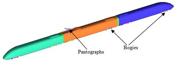
This paper took a high-speed train as the researched object and selected 3-train formation including head train, tail train and middle train with pantograph. Each train contained two bogies. As the train body was not smooth, the model was simplified and some parts with small dimensions were removed. The windshield at the junction of train body planned to be outsourced. The simplified model of train was shown in Fig. 1. Head train and tail train were set symmetrically. According to the dimension parameters of train, length, width and height were 76.55 mm, 3.26 m and 3.64 m, respectively.

Fig. 1Three-dimensional geometry model of high-speed trains

3.2. Computational domain

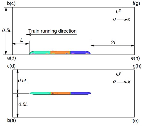
The computational domain of aerodynamic noises of high-speed trains was shown in Fig. 2. Train length $L=$76.55 m was taken as the benchmark. Therefore, the length, width and height of computational domain were 4$L$, $L$ and 0.5$L$. The distance between the nose tip of head train and fluid entrance was $L$; the distance between the nose tip of tail train and fluid exit was 2$L$; the distance between the train and the ground connected with track was 0.2 m. Cross sections abcd right in front of the high-speed train were inlet boundaries and set as velocity inlet conditions. In the case of computation, velocities were 300 km/h (83.3333 m/s) and 400 km/h (111.1111 m/s). Cross sections efgh right behind the high-speed train were outlet boundaries and set as pressure outlet conditions. It was 1 standard atmospheric pressure. Cross sections bfgc right above the high-speed train, cghd at the left side of the high-speed train and aefb at the right side of the high-speed train were set as symmetric boundary conditions. The surface of high-speed train was set as fixed boundary. It was no-slip wall boundary condition. To simulate ground effect, grounds aehd were set as slip grounds, whose slip velocity was the running speed of the high-speed train.

Fig. 2Computational domain of the high-speed train

3.3. Meshes of the high speed train

ICEM CFD was adopted to divide meshes. Unstructured meshes were selected. The maximum size of flow field was 1500 mm; the biggest mesh of train surface was 60 mm; the biggest mesh of pantograph was 10 mm; the biggest mesh of bogies was 30 mm; the biggest mesh at the surface of air conditioning was 40 mm. Train body, bogies and pantograph surface adopted triangular meshes. The size of three-dimensional meshes was amplified according to a certain scale factor. Hexahedral meshes were used at the places far away from train body. The transition from tetrahedral meshes to hexahedral meshes adopted pentahedral pyramid meshes. The total number of meshes was about 74,220,000, and the model was shown in Fig. 3.

Fig. 3Meshes of the high-speed train

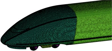
a) Head train

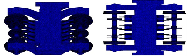
b) Bogies

4. Aerodynamic flow behavior of high-speed trains

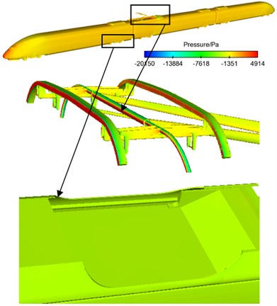
Fig. 4 displayed the contour of pressure at the surface of the high-speed train when it ran at the speed of 300 km/h. As shown in Fig. 4(b), the maximum pressure of head train was at the position of nose tip and it was 4427 Pa. The maximum negative pressure was in the part of cowcatcher and it was 10578 Pa. This was due to that the stagnation speed at the nose of the head train was 0 and the airflow at the nose was separated, so that the positive pressure at the nose position of the head train was the maximum. Due to the resistance on the wind side of the exhaust barrier of the head train, airflow separation presented on the wind side of the exhaust barrier of the head train and quickly flowed into the bogie area, so that the negative pressure at the leeward side of the head train was the maximum. As displayed from Fig. 4(c), the maximum positive pressure of tail train was at the window of driver’s cabin and it was 1816 Pa, which was caused by the window of the tail train. The maximum negative pressure was at the leeward side of air conditioner in tail train and it was 6148 Pa. The maximum positive pressure of the whole train was at the windward side of pantograph head and it was 4914 Pa. This was due to that the section in the skateboard of the pantograph head of pantographs was rectangle, and the nose in the wind side of the skateboard was the blocking surface, so that it was the maximum positive pressure position at the surface of the whole train. The maximum negative pressure of the whole train was in bogie area and it was 20150 Pa. This was due to that turbulence was in the bogie area, and the vortex was very complex, so that the maximum negative pressure was in the bogie area including air conditioner.

Fig. 4Contours of pressure at the surface of high-speed trains

a) The whole train

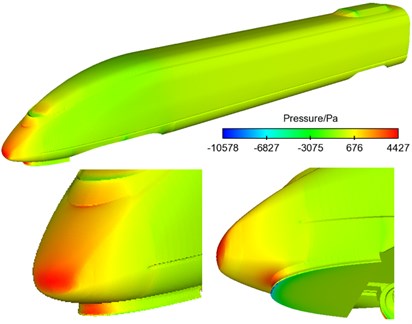
b) Head train

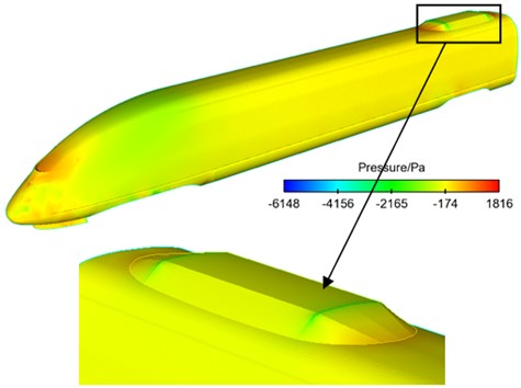
c) Tail train

The aerodynamic noise source of high-speed trains was mainly dipole noises. Dipole sound source was determined by the fluctuating pressure of train surface [10]. Namely, the size of fluctuating pressure at the surface of train body could be used to reflect the situation of noise radiation at the surface of sound generation. According to three control equations, turbulent kinetic energy equation and turbulent dissipation rate equation of flow field, the size of fluctuating pressure at the surface of train body could use turbulent kinetic energy $k$ to assess the distribution characteristics of noises at train surface.

Fig. 5 displayed the distribution of turbulent kinetic energy at the surface of high-speed trains and pantograph area. As shown in Fig. 5, the distribution area of high turbulent kinetic energy was in the position of transition between the nose tip and non-streamlined position of head train, between windshield at first end of train and pantograph area, between air conditioning and pantograph area, between pantograph area and windshield at the second end of train. In addition, turbulence at the front end of pantograph air deflector shocked pantograph, which resulted in the large noise in pantograph. Turbulence continued to shock the rear of pantograph area. In addition to the vortex shedding of pantograph, noise radiation in pantograph area was further increased. In a similar way, high turbulent kinetic energy area also existed in the position of windshield at A end of car, which indicated that windshield at A end of car was also the distribution area of main noise source. Thus, it could be seen that pantograph, pantograph area, nasal tip of head car, cowcatcher part of head car, bogie area and windshield area were main noise sources of high-speed train. Additionally, the sound source areas of high-speed train were at places where airflow would be separated easily and turbulence moved violently.

Fig. 5Contours for the distribution of turbulent kinetic energy of high-speed trains

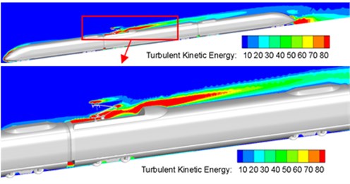
a) The whole train

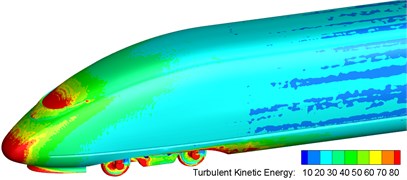
b) Head train

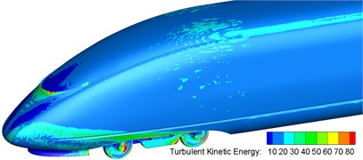
c) Tail train

Fig. 6 displayed the distribution of vorticity contour surface based on Q-criterion (Dimension was 0.001) when the high-speed train ran at the speed of 300 km/h. As displayed from Fig. 6, main vortexes were in the streamlined area of head train, bogie area, windshield area, pantograph area, air deflector area of air conditioners and non-streamlined area of tail train. Similarly, it could be seen that main aerodynamic noise sources were in pantograph, pantograph area, head streamlined area, bogies, bogie area, windshield area, area of air conditioning and other areas. Thus, the vortex shedding and fluid separation of the whole train were main reasons for the aerodynamic noise of the whole train. As displayed from Fig. 6(b), vortexes in pantograph and pantograph area were more violent than those in other areas. There were large vortexes in pantograph head, junction of upper arm and lower arm and chassis area, which indicated that this area was the main aerodynamic noise source of pantograph. Similarly, large vortexes could be found in pantograph tail, which showed that pantograph area was also the main aerodynamic noise source of the whole train and main aerodynamic noise source was in places where the curvature of components witnessed great changes or vortexes drastically changed. As displayed from Fig. 6(c) and Fig. 6(d), the vortex distribution of bogie area at the first end of head train showed a wider range than that at the first end of tail train. Therefore, bogie at the first end of head train was the main aerodynamic noise source of the whole train compared with other bogies.

Fig. 6Distribution diagram of vorticity of high-speed trains

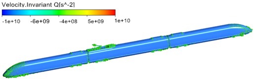
a) The whole train

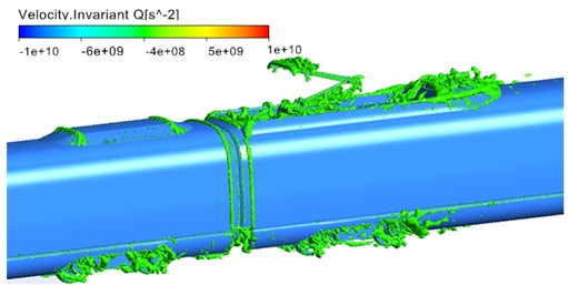
b) Pantograph area

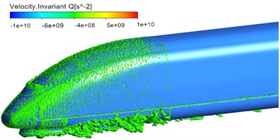
c) Head train

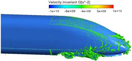
d) Tail train

5. Aerodynamic noise characteristics of high-speed trains

5.1. Analysis on fluctuating pressure at the surface of high-speed trains

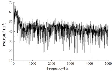
Researches showed that the aerodynamic noise of high-speed trains was mainly determined by the fluctuating pressure of body surface [13]. Therefore, it was necessary to analyze the change rule of fluctuating pressure at the surface of train body. When the train ran at a certain speed, a comparative analysis was conducted on the fluctuating pressure of various observation points to find that fluctuating pressure in the streamlined part of head train had a great change [13]. Fluctuating pressure at the nose tip of head train reached the maximum. It was because airflow flowing through the nose tip of the train was separated. A part of airflow flowed upward along the surface of train body while a part of airflow flowed downward along the bottom, which resulted in the most intense airflow disturbance and separation in the nose tip of the train. As a result, this paper took the observation point of nose tip of head train as an example to analyze the time-domain and frequency-domain characteristics of fluctuating pressure. Fig. 7 showed the time-domain curve of fluctuating pressure at the observation point of nose tip of head train when the running speed of train was 300 km/h. Fig. 8 was the corresponding power spectrum density.

As displayed from Fig. 7 and Fig. 8, pressure at the body surface of high-speed trains fluctuated randomly and showed irregular changes in the time domain. Fluctuating pressure of body surface was broadband signals in the frequency domain and its energy was mainly in the low frequency. With the scope of 800 Hz, power spectrum density dropped quickly with the increase of frequency. When the analyzed frequency was higher than 1000 Hz, power spectrum density will be stable and changed little.

Fig. 7Fluctuating pressure at the observation point of nose tip of head train

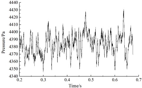
Fig. 8Power spectrum density at the observation point of nose tip of head train

5.2. Distribution characteristics of longitudinal aerodynamic noise of high-speed train

Fig. 9 displayed the comparison curve of sound pressure levels at longitudinal observation points when the high-speed train ran at the speed of 300 km/h and 400 km/h, respectively. These observation points were 25 m away from the center line of track and 3.5 m away from rail surface. 78 noise observation points were distributed longitudinally along the train. The distance between two adjacent longitudinal observation points was 1 m [26, 27]. As displayed from Fig. 9, the distribution of sound pressure level of longitudinal aerodynamic noises of high-speed trains presented a decreasing trend. The sound pressure level in the back of bogies at the first end of head train reached the maximum value. In the back of bogies at the first end of head train, total sound pressure level reached the maximum value. Total sound pressure levels were the maximum in bogie area at the second end of head train, bogie at first end of middle train, bogie area at second end of middle train, bogie area at the second end of tail train and bogie at the first end of tail train. When the nose tip of head train changed into $x=$12 m, the sound pressure level of noises increased by 17.1 dBA at most. Then, the noise sound pressure level of the whole train changed little. When the nose tip of head train changed into $x=$12 m, the sound pressure level of noises reached the maximum value among all observation points of the whole train, namely 96.5 dBA. In the streamlined part of tail train, sound pressure levels decreased rapidly and the maximum attenuation value was 9.2 dBA. In the same way, total sound pressure levels reached local maximum values around bogie at the second end of head train, bogie at the first end of middle train, bogie at the second end of middle train and bogies at the first and second ends of tail train. Maximum sound pressure levels were 93.2 dBA, 93.3d BA, 92.2 dBA, 91.9d BA and 93.5 dBA, respectively.

From the comparative analysis of Fig. 9, the sound pressure level of longitudinal observation points increased obviously with the increase of running speed of train. When the running speed of train was 400 km/h, sound pressure levels reached the maximum value among all observation points of the whole train in the case of $x=$12 m, namely 101.4 dBA. Maximum sound pressure levels were 97.9 dBA, 98.3 dBA, 97.2 dBA, 96.9 dBA and 98.3 dBA, respectively around bogie at the second end of head train, bogie at the first end of middle train and bogie at the second end of middle train, bogie at the first and second of tail train. When the running speed was 300 km/h and 400 km/h, the maximum sound pressure level of the whole train has increased by 4.9 dBA.

Fig. 9Sound pressure levels under different running speeds

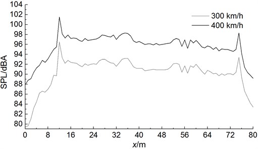
Fig. 10 displayed the comparison of high-speed trains at observation points under one-third octave (the position of longitudinal maximum sound pressure level). As shown in Fig. 10, aerodynamic noises of high-speed trains were a wide frequency spectrum which was a kind of broadband noise and whose main energy was within the frequency of 1000 Hz to 4000 Hz. With the increase of running speeds, its aerodynamic noise energy moved to the high frequency. The computational result was also compared with the experimental result from reference [28]. The change trend was similar and the difference is also small in the high frequency because noises were main the aerodynamic noise in the high frequency. However, the noise included mechanical noises and aerodynamic noises in the low frequency, so the computational result was smaller than that of the experiment.

5.3. Distribution of aerodynamic noises in pantograph area

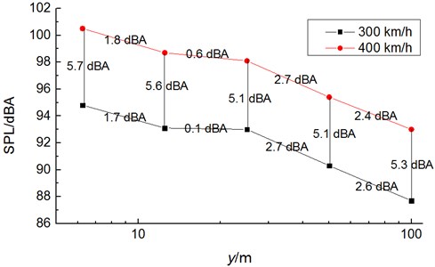
5 noise observation points were distributed horizontally ($y$-axis) along the train at places which were 3.5 m from the track, 48 m away from the nose tip of head train and 6.25 m, 12.5 m, 25 m, 50 m and 100 m (The distance between two adjacent observation points was double) away from pantograph area. Fig. 11 displayed the comparison of sound pressure levels at noise observation points of pantograph area when the high-speed train ran at the speed of 300 km/h and 400 km/h. As displayed from Fig. 11:

(1) Attenuation amplitudes of horizontal noises at 5 observation points were 1.7 dBA, 0.1 dBA, 2.7 dBA and 2.6 dBA, respectively when the high-speed train ran at the speed of 300 km/h.

(2) Attenuation amplitudes of horizontal noises at 5 observation points were 1.8 dBA, 0.6 dBA, 2.7 dBA and 2.4 dBA, respectively when the high-speed train ran at the speed of 400 km/h. Therefore, the total sound pressure levels of two adjacent observation points whose distance was double decreased by 2.7 dBA when $y=$25 m.

(3) Attenuation amplitudes of horizontal noises at 5 observation points were 5.7 dBA, 5.6 dBA, 5.1 dBA, 5.1 dBA and 5.3 dBA respectively when the high-speed train ran at the speed from 300 km/h to 400 km/h.

Fig. 10A comparative analysis on aerodynamic noises under one-third octave

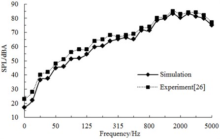
a) 300 km/h

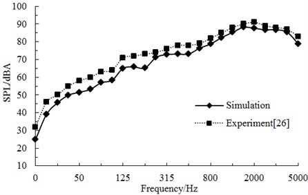
b) 400 km/h

Fig. 11A comparison curve of sound pressure levels in pantograph area

5.4. Propagation characteristics of aerodynamic noises of pantograph

It was found that pantograph was the main aerodynamic noise source of high-speed trains through analysis. Therefore, this paper would study the radiation characteristics of aerodynamic noises of pantograph when the running speed of train was 300 km/h. This paper extracted the time-domain signals of fluctuating pressure of pantograph from the flow field and adopted the boundary element method to solve sound pressure. In addition, this paper adopted acoustic software Virtual.Lab to compute acoustic propagation at the surface of pantograph, used sound pressure boundary conditions to map fluctuating pressure of pantograph to the acoustic meshes, applied Discrete Fourier Transform (DFT) to transfer the data of surface fluctuating pressure, conducted acoustic response computation and obtained the radiation characteristics of aerodynamic noises of pantograph. Fig. 12 showed the acoustic meshes of pantograph and the biggest mesh size satisfied the requirement of maximum frequency. Fig. 13 displayed a comparison of noise radiation of aerodynamic noises at the frequency of 500 Hz, 1000 Hz and 2000 Hz.

According to the comparative analysis of Fig. 13, the aerodynamic noise of pantograph of high-speed trains was mainly distributed in the mid-high frequency and aerodynamic noise energy in low-frequency was lower than that in high-frequency. The main radiation direction of aerodynamic noises of pantograph was the upper left and right at 500 Hz when the running speed was 300 km/h. The main radiation direction of aerodynamic noises was right above at 1000 Hz, and both sides were not main radiation directions of aerodynamic noises. At 2000 Hz, the main radiation direction of aerodynamic noises was the upper left and right. Main energy in this position was more intense than that at 500 Hz, which was mainly attributed to the contribution of pantograph head to the radiation energy of aerodynamic noise. As a result, the contribution of aerodynamic noises of pantograph was mainly from pantograph head. Thus, the noise reduction effect of pantograph head would be the most obvious if low-noise optimization design was conducted for pantograph head subsequently.

Fig. 12Acoustic meshes of pantograph

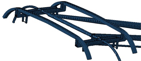
Fig. 13Contours of the aerodynamic noise radiation of pantograph

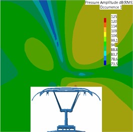
a) 500 Hz

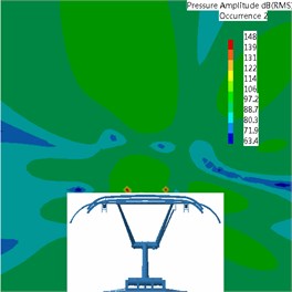
b) 1000 Hz

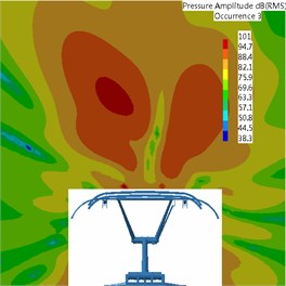
c) 2000 Hz

6. Conclusions

Based on Lighthill acoustic theory, this paper adopted LES and FW-H acoustic model to conduct numerical computation for the aerodynamic noise of high-speed trains, analyzed the aerodynamic flow behavior and aerodynamic noise characteristics of high-speed trains, considered the aerodynamic model of microscopic structures (pantograph, pantograph area, bogie, air conditioning, junction of train ends and so on) of train in the case of modeling, established a computational model for the aerodynamic noise of 3 train formation, and came to the following conclusions:

1) Pantograph, pantograph area, streamlined area, bogies, bogie area, windshield area, and air conditioning area were main aerodynamic noise sources of high-speed trains. The main aerodynamic noise source of pantograph was mainly distributed in pantograph head, junction of upper arm and lower arm and chassis area. Compared with other 5 bogies, bogie at the first end of head train was main aerodynamic noise source. In addition, vortex shedding and fluid separation were main reasons for the aerodynamic noise of high-speed trains.

2) Through conducting a comparative analysis on the total sound pressure level of observation points (25 m away from the center line of track and 3.5 m from the rail surface) of high-speed trains, this paper found that the total sound pressure level of observation point which was 12 m away from the nose tip of head car was the maximum. The maximum value was 96.5 dBA when the high-speed train ran at the speed of 300 km/h. The maximum value was 101.4 dBA when the high-speed train ran at the speed of 400 km/h. In the direction of the operation, the distribution curve of longitudinal sound pressure levels showed local maximum sound pressure levels in bogies at the first and second ends of head train, middle train and tail train. To reduce the total sound pressure level of the whole train, this paper suggested focusing on taking noise reduction measures in 6 positions. The noise reduction effect of the whole train should be very obvious.

3) With wide frequency spectrum, the aerodynamic noise of high-speed trains was a kind of broadband noise, whose main energy was mainly within the frequency of 1000 Hz to 4000 Hz. With the increase of speeds, the aerodynamic noise energy moved to the high frequency.

4) The distribution of aerodynamic noises in pantograph area had the following characteristics: the total sound pressure level of two adjacent observation points whose distance was double decreased by 2.7 dBA when $y=$25 m; the average attenuation amplitude of sound pressure levels at various horizontal observation points of high-speed trains was 5.4 dBA when the running speed of high-speed trains increased from 300 km/h to 400 km/h.

5) Propagation of aerodynamic noises of pantograph had the following characteristics: The main radiation energy of pantograph was in mid-high frequency and its main radiation direction was at the upper left and right sides of pantograph head. In the high frequency, the contribution of aerodynamic noises of pantograph mainly came from pantograph head.