Numerical simulation and experimental study of aerodynamic noises for the cabin of the high-speed train

Lv, Ming; Xu, Dong-er; He, Hua

doi:10.21595/jve.2016.17140

Journal of Vibroengineering

Browse Journal

Submit article

Published: 15 February 2017

Check for updates

Numerical simulation and experimental study of aerodynamic noises for the cabin of the high-speed train

Ming Lv¹

Dong-er Xu²

Hua He³

^{1, 2, 3}School of Mechanical and Vehicle Engineering, Bengbu University, Bengbu, 233000, China

Corresponding Author:

Ming Lv

Cite the article Download PDF

Downloads 1321

Abstract

For improving noises in the cabin quickly, large eddy simulation was adopted to compute the fluctuating pressure of the cabin surface numerically. Then, the fluctuating pressure was mapped to the boundary element model as the excitation loads to obtain the aerodynamic noise distribution of the cabin at different frequencies, which was then compared with the experimental result. There were some differences between the computational model and actual model, and the experimental results were more than the simulation result, which was within the acceptable range of the engineering. The comparative result indicated that the prediction model was reliable. In addition, as presented from the computational results: SPLs on cabin surface were changed between 60-110 dB, and greater SPLs were located on the transition position which was from the nose tip to the roof surface of the cabin. The aerodynamic noise on the cabin surface was mainly in low-frequency.

1. Introduction

The dynamic environment of the high-speed train was changed into the aerodynamic force, which brought serious change and restriction of excessive noise pollution, therefore being rejected in a veto [1]. S2500 train reached 350 km/h in both design and experimental speeds. However, it was limited by noises, and the train was only allowed to operate at the speed of 300 km/h. Therefore, the control of noises was the necessary requirement for the realization of the sustainable and development of the railway. Aerodynamic noises were increased with the sixth power of the train speed [2]. With the constant construction of the high-speed railway and further increase of the speed, the aerodynamic noise was becoming more and more prominent. Therefore, the research and reduction regarding aerodynamic noises has become the key to controlling the high-speed train noise. Through wind tunnel test and numerical simulation, the aerodynamic noise source and external fluctuating pressure of the high-speed train were studied and the analysis of the external sound field was conducted [3-5]. Liu solved the generalized Lighthill equation, obtained integral formulas of the aerodynamic noise, and made experimental research on the distribution and frequency characteristics of the fluctuating pressure in the wind tunnel [6, 7]. Liu also established mathematical and physical model for three-dimensional circumferential flow field regarding the head of the high-speed train, applied Lighthill acoustic analogy theory to compute the far-field aerodynamic noise of the high-speed train, and adopted a broadband noise source model to compute the aerodynamic noise source on the body surface of the high-speed train [8]. Xiao used the head surface of the high-speed train as the research object and analyzed aerodynamic noise characteristics of the head [9]. Yuan established a computational model including a head train and a tail train, in order to computing aerodynamic noise source intensity and far-field aerodynamic noises on the train surface [10]. A computational model including a head train, middle train and tail train was built in reference [11] to compute noise source intensity and far-field aerodynamic noise on the train surface, although the detailed analysis and summary did not consider bogies and far-field noises in the model. Sun established the aerodynamics model of the high-speed train, analyzed the flow field characteristics of the train head, compartment joint and train tail, and studied the contribution of different train parts on the aerodynamic noise, which ignored bogies and pantographs [12].

The mentioned study ignored the train floor and porous sound absorption materials when the aerodynamic noise model of the high-speed train was established, whose model accuracy was therefore not very high. Besides, the researched object was the entire train model, which would reduce the computational efficiency and increase the computational cost. Only aerodynamic noises of the high-speed train cabin were studied in the paper. When the aerodynamic noise model of the cabin was established, the interior trims of the train were considered, and then only the local model of the head was established for researches, which could improve the computational efficiency and cost.

2. Computational method of aerodynamic noises of the high-speed train

2.1. Main transmission process of aerodynamic noises

When the high-speed train was operating, the train interacted with the air. In several parts of the body, the airflow emerged separation vortex and vortex shedding, thus generating unsteady flow. Therefore, strong fluctuating pressure field was appeared on the external surface of the body. The fluctuating pressure acting on the exterior surface of the body was the reason of the interior aerodynamic noise [8]. Exterior fluctuating pressure and the induced aerodynamic noise had two main transmission ways to the train [9]: Firstly, exterior aerodynamic noises spread to the train through the door, windows and another gap directly. Secondly, external fluctuating pressure acted on the train panels, doors and windows, caused the vibration of panels, doors and windows and radiated noises to the interior space. When the closure condition of the train was good, the noise transmitted through holes and pores can be ignored. Therefore, the vibration was the main noise source. Two stages were conducted during the computation of the aerodynamic noise of the cabin: large eddy simulation was applied to compute the transient external flow field of the cabin surface and obtain the fluctuating pressure; and boundary element method was adopted to compute the aerodynamic noise.

2.2. Control equations of large eddy simulation

Large Eddy Simulation (LES) had the basic idea to compose the turbulent flow through different scales of eddies. And large-scale eddy played a major role in the generation of turbulence energy and Reynolds stress as well as diffusion of various turbulence amounts. The behavior of large eddy was strongly dependent on the boundary conditions, which varied in accordance with the flow type. However, small vortex had small impact on the trend of above functions, and the minimum eddy primarily played the dissipation role. At high Reynolds number, the small eddy was approximately isotropic and less affected by the boundary conditions, with greater commonality. Although dissipation scale cannot be computed through the current computer, inertial scale can be obtained. Therefore, N-S equations which were relevant to the discrete time could be applied to determine the behavior of big eddy, and more general model could be adopted to simulate the behavior of small vortex. Furthermore, the flow field speed variable $u_{i}$ in N-S equation was changed to the large scale through LES to solve the variable ${\bar{u}}_{i}$ directly. Thus, flow field variables can be decomposed into two parts of large scale and subgrid scale, as shown below:

1

u_{i} = {\bar{u}}_{i} + u_{i}^{'},

wherein: $u_{i}^{'}$ was the filtered subgrid scale, and ${\bar{u}}_{i}$ was the big eddy greater than the filter scale, which was obtained in the whole computational domain $D$ through the following convolution integral:

2

{\bar{u}}_{i} (x_{1}, x_{2}, x_{3}) = ∭_{D} [\prod_{j = 1}^{3} G_{j} (x_{j}, x_{j}^{'})] u_{i} (x_{1}^{'}, x_{2}^{'}, x_{3}^{'}) d x_{1}^{'} d x_{2}^{'} d x_{3}^{'},

wherein: $x_{i}$ and $x_{1}^{'}$ were spatial coordinates, and $G$ was the filter function, which satisfied the following equation:

3

∭_{D} [\prod_{j = 1}^{3} G_{j} (x_{j}, x_{j}^{'})] d x_{1}^{'} d x_{2}^{'} d x_{3}^{'} = 1 .

The filter with volume-weighted function was most commonly applied in the finite difference method and finite volume method, namely:

4

G_{j} (x_{j}, x_{j}^{'}) = \{\begin{array}{l} 1 / Δ_{j}, \begin{array}{l} |x_{j} - x_{j}^{'}| \leq Δ_{j} / 2, \end{array} \\ 0 \begin{array}{l} \begin{array}{l}  \end{array} & |x_{j} - x_{j}^{'}| > Δ_{j} / 2, \end{array} \end{array}

wherein: $Δ_{j}$ ( $j =$ 1, 2, 3) was the grid scale in three coordinate directions. After filtering, the obtained incompressible N-S equation form was as follows:

5

\frac{\partial {\bar{u}}_{i}}{\partial t} + \frac{\partial (\bar{u_{i} u_{j}})}{\partial x_{j}} = - \frac{1}{ρ} \frac{\partial \bar{p}}{\partial x_{i}} + υ \frac{\partial^{2} {\bar{u}}_{i}}{\partial x_{k} \partial x_{k}},

wherein: $ρ$ , $υ$ were air density and kinematic viscosity, respectively. ${\bar{u}}_{i}$ , $\bar{p}$ were the filtered speed and pressure, respectively. As ${\bar{u}}_{i}$ and $\bar{u_{i} u_{j}}$ cannot be solved simultaneously, the following decomposition need to be made: $\bar{u_{i} u_{j}} = {\bar{u}}_{i} \cdot {\bar{u}}_{j} + τ_{i j}$ . Wherein, $τ_{i j}$ was the subgrid shear stress tensor, $τ_{i j} = τ_{k k} δ_{i j} / 3 - 2 μ_{t} {\bar{S}}_{i j}$ , and $μ_{t}$ were subgrid turbulence viscosity. ${\bar{S}}_{i j}$ was the strain rate tensor determined by the solved large eddy, which can be expressed as follows:

6

{\bar{S}}_{i j} = \frac{1}{2} (\frac{\partial {\bar{u}}_{i}}{\partial x_{j}} + \frac{\partial {\bar{u}}_{j}}{\partial x_{i}}) .

The incompressible N-S equation with continuity equation can be expressed as follows:

7

\frac{\partial {\bar{u}}_{i}}{\partial x_{i}} = 0,

8

\frac{\partial {\bar{u}}_{i}}{\partial t} + \frac{\partial {\bar{u}}_{i} {\bar{u}}_{j}}{\partial x_{j}} = - \frac{1}{ρ} \frac{\partial \bar{p}}{\partial x_{i}} + υ \frac{\partial^{2} {\bar{u}}_{i}}{\partial x_{k} \partial x_{k}} - \frac{1}{ρ} \frac{\partial τ_{i j}}{\partial x_{j}} .

In the application of Smagorinsky model, the subgrid turbulence viscosity can be expressed as the following equation:

9

μ_{t} = ρ L_{s}^{2} |\bar{S}|,

wherein: $|\bar{S}| = \sqrt{2 S_{i j} S_{i j}}$ , subgrid mixing length was $L_{s} = m i n (k δ, C_{s} V^{1 / 3})$ , $k =$ 0.42 was a parameter of von Karman, $δ$ was the distance to the nearest wall, $V$ was the volume of the computed element, $C_{s}$ was Smagorinsky constant, and $C_{s} =$ 0.1 can give a reasonable solution in a wide flow range.

2.3. Control equations of the acoustic boundary element method

The displacement response of the train was a time-domain response under aerodynamic loads, which could obtain the frequency-domain response of the structural displacement after Fourier transformation. The sound field pressure $p$ should meet the Helmholtz equation:

10

\nabla^{2} p - k^{2} p = - j ρ_{0} ω q,

wherein: $k$ was the wave number, $j$ was the imaginary unit, $ρ_{0}$ was the air density, $ω$ was the angular frequency, and $q$ was the volume velocity per unit volume.

In the fluid-solid surface $S$ , the solution $p$ of Helmhotz equation should satisfy the following equation:

11

\partial p / \partial n = - j ρ ω υ_{n},

wherein: $n$ was the normal direction of the border, and $υ_{n}$ was the normal speed on surface $S$ .

The sound pressure $p$ at any point of interior sound field of the train can be obtained through the integration of sound pressure $p$ on surface $S$ and normal vibration velocity $υ$ , namely:

12

p = C^{T} p + D^{T} υ,

where: $C_{i}$ and $D_{i}$ were components of $C$ and $D$ , respectively:

13

C_{i} = \int_{S} N_{i} \times \frac{\partial G (X, Y)}{\partial n} d S,

14

D_{i} = j ρ_{0} ω \int_{S} N_{i} \times G (X, Y) d S,

wherein: $N_{i}$ was the shape function, which was 1 on node $i$ and 0 on other nodes. $G (X, Y)$ was the Green function, which should satisfy the Helmholtz equation.

3. Computation of aerodynamic characteristics of the high-speed train

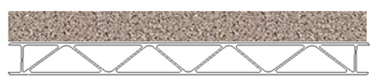
The body structure of the high-speed train was consisted of the aluminum profile, as shown in Fig. 1. It included aluminum profiles of roof, floor and lateral side, respectively. Then, some sound absorption materials were installed on the aluminum profile to form the interior trims of the high-speed train, as shown in Fig. 2.

Fig. 1Aluminum profiles of body structure

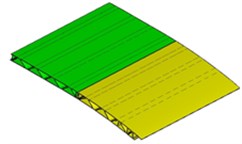
a) Roof aluminum profile

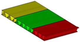
b) Floor aluminum profile

c) Lateral side aluminum profile

Fig. 2Interior trims of the high-speed train

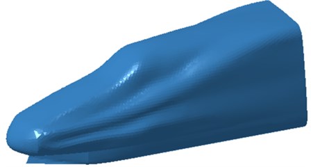
The paper mainly researched aerodynamic noises on the surface of the high-speed train cabin and did not pay attention to noises in the passenger compartment. When the aerodynamic noise of the high-speed train was researched, appendixes such as bogies and pantographs were always ignored, so that the top and bottom parts of the train were approximated as plane structures. When flow passed through the train top and bottom, it can realize smooth transition and would not be influenced by any outstanding object in general. Therefore, the vortex field at the tail part of the truncated model was kept basically consistent with that of the complete model. Therefore, the paper only researched the cabin model. In addition, the vortex field in the tail would not influence the noise in cabin. In addition, by applying the truncated model in the research, the computational time can be saved, and the computational efficiency can be improved. At present, this method has been adopted in some published papers. For example, Xiao [13] used a truncated model to research the aerodynamic noise in a high-speed train cabin. However, the research results in reference [13] were not refined and verified by experiments.

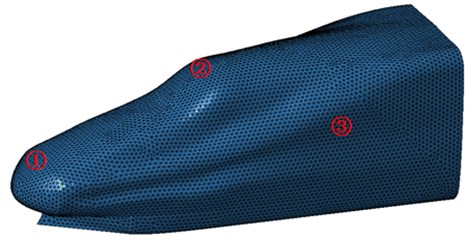
The high-quality element was critical for improving the computational precision regarding transient flow field of the head surface and improving the convergence process. The structural element based on the mapping method was featured with high computational efficiency and ordered arrangement, thus being an ideal meshing method. According to quadrilateral mesh method of the head generated by the mapping method, the three-dimensional modeling software CATIA was adopted to output the appearance of complex high-speed train as the mapping reference, and the quadrilateral element was mapped to the streamlined shape surface of the high-speed train, which could save the simplification process for the streamlined shape and could divide elements very orderly. Based on the generated quadrilateral element of the high-speed train surface, a hexahedral mesh used for flow field could be formed easily. The geometric model can be found in Fig. 3. The fluctuating pressure on the train surface was relatively small when the analyzed frequency was more than 1000 Hz [10]. Therefore, the maximum computation frequency was set as 1000 Hz when the flow field around the train head was simulated numerically by LES method. In the computation, the fluctuating pressure of each node on the body surface was monitored. Strong pressure gradient was in the nose tip, in the lower front window of the cabin, and in the transition position from the head surface to the roof. Therefore, in the lines of the longitudinal symmetrical plane of the head surface, three observation points were selected in the nose tip, in the lower front window of the cabin, and in the transition position from the head surface to the roof as key objects for discussions.

Fig. 3Geometric model of the high-speed train cabin

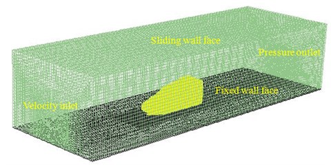
Based on the finite volume method, the commercial software Fluent was applied for analysis and adopted to make numerical simulation of unstructured elements. The turbulent flow was solved based on LES in Fluent framework and through the application of Smagorinsky-Lilly subgrid model. The non-viscidity condition was applied in two lateral sides, sliding boundary condition was applied in the roof surface, and fixed boundary condition was applied in the floor. The inlet of the computational domain was designated as the velocity inlet, whose speed was set as 250 km/h. Such speed was corresponding to the Reynolds number $R_{e} =$ 1.23×10⁷. The outlet was designated as the pressures outlet, as shown in Fig. 4. The outer surface of the cabin was extracted to obtain the flow elements using HYPERMESH. Flow elements on the outer surface were triangular element, and there were 50672 elements and 57825 nodes. The material was steel, and elastic modulus was 2.1e¹¹, density was 7.8e³kg/m³, and Poisson’s ratio was 0.31.

RANS framework could be applied for the computation, in order to realize the $k$ - $ε$ eddy viscosity transmission model and obtain the steady solution of the flow field. Based on such steady solution, LES was applied for the unsteady computation of the flow field. In consideration of two factors of the computational accuracy and efficiency, the unsteady time step was determined as 5×10⁴ s, and twenty-five sub-iterations were conducted each time. Through the analysis of residuals, the pressure coefficients of rear mirror and body surface, rear mirror speed and other parameters can be monitored, the computational convergence in each time step was determined, and sufficient sample points in the quasi-periodic flow could be ensured by the set time step. The process of change regarding observation points at 0-1 s was analyzed, finding that dynamic steady flow was determined in the computational time of more than 1 s. A total of 4000 time steps were required for the entire computation, and the results of the final 2000 time steps were applied for the unsteady data analysis. It should be noted that the time step required for the computation can ensure the enough points of all observation points in the quasi-periodic period. Meanwhile, the analysis of the final 1 s data can guarantee that standard values of average pressure factor and fluctuating pressure factor brought from the computation had the maximum error of 0.5 %.

Fig. 4Computational domain of the high-speed train cabin

The fluctuating pressure $P_{v}$ on the train surface was related to the pulsating pressure level. The fluctuating pressure level $L_{v}$ was defined as follows:

15

L_{v} = 10 l g {(P_{v} / P_{0})}^{2},

wherein: $P_{0}$ was the reference pressure with the value of 2×10⁵ Pa.

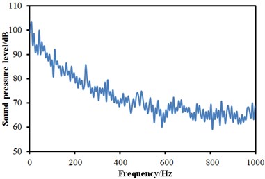
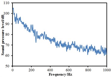
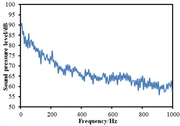
The fluctuating pressure level obtained through Eq. (15) was shown in Fig. 5. It was indicated that the fluctuating pressure level at observation point 1 and point 2 was significantly greater than that at observation point 3. And obvious peaks and valleys were presented in the fluctuating pressure level at various observation points. The pressure contours of the high-speed train cabin at 0.125 s, 0.250 s, 0.375 s and 0.500 s were extracted as shown in Fig. 6. As presented in Fig. 9, the relatively large pressure was mainly appeared in the transition position and at the bogie. Fig. 7 was the velocity contour of the high speed train cabin. With the increase of the analyzed time, the velocity in the tail of the high speed train has an obvious change.

4. Computation of aerodynamic noises of the high-speed train

Acoustic analysis software Virtual.lab was applied in the paper to establish an acoustic boundary element model of the high-speed train cabin. Due to the unavailable modeling capabilities in the pretreatment of Virtual.lab software, the finite element model of sound field of the cabin cavity was firstly established in HYPERMESH and then imported to the Virtual.lab in BDF format. Before modeling, the size of acoustic elements should be determined; whose ideal size was approximately six elements in each wavelength. The boundary element model of the high-speed train cabin was finally obtained as shown in Fig. 8.

Fig. 5Fluctuating pressure level at three observation points

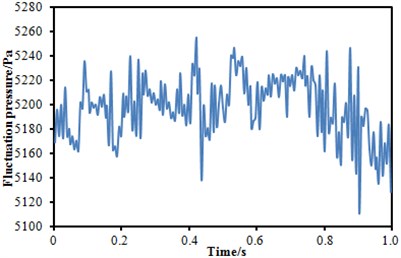
a) Fluctuating pressure level at point 1

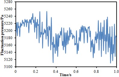
b) Fluctuating pressure level at point 2

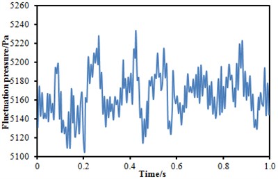
c) Fluctuating pressure level at point 3

Fig. 6Fluctuating pressure contours of the high-speed train cabin

a) 0.125 s

b) 0.250 s

c) 0.375 s

d) 0.500 s

Fig. 7Velocity contours of the high-speed train cabin

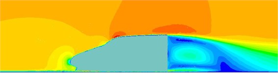
a) 0.125 s

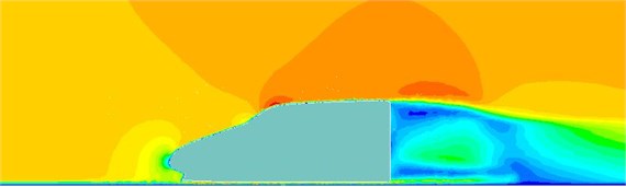
b) 0.250 s

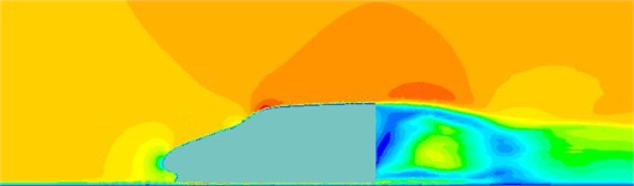
c) 0.375 s

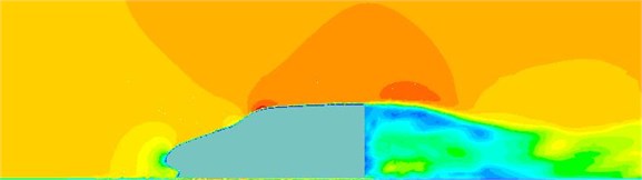
d) 0.500 s

Fig. 8Boundary element model of the high-speed train cabin

The aerodynamic characteristics in Section 3 were imported into Virtual.lab and the computational result was mapped to the boundary element meshes. Therefore, all characteristics of structural meshes could be obtained through acoustic elements, thereby obtaining acoustic results. Similarly, three observation points were arranged at the cabin nose tip, in the transition position from the nose tip to the roof and in the windows, and their SPLs were extracted, as shown in Fig. 9. It could be seen that SPLs at the observation points 1 and 2 were significantly larger than that of observation point 3. In addition, SPLs at all observation points were gradually decreased with the increase of the analyzed frequency. There were no any obvious peaks in the whole observation point. The minimum of the observation point 1 was 62.2 dB and the corresponding frequency was 587 Hz. The minimum of the observation point 2 was 63.3 dB and the corresponding frequency was 947 Hz. The minimum of the observation point 3 was 57.1 dB and the corresponding frequency was 923 Hz.

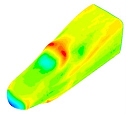
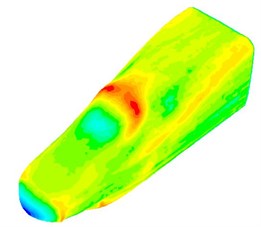
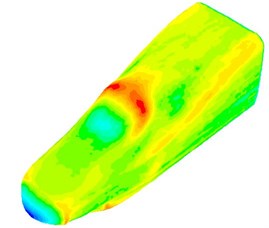
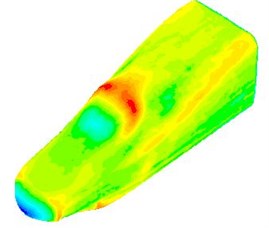
The SPL contours at 100 Hz, 300 Hz, 500 Hz and 700 Hz were extracted, whose results were shown in Fig. 10. It was indicated that greater SPLs were presented in transitions and bogies, which was consistent with the above result of aerodynamic characteristics.

Fig. 9SPLs curves at three observation points

a) SPLs at observation point 1

b) SPLs at observation point 2

c) SPLs at observation point 3

Fig. 10SPL contours of the high-speed train cabin

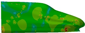
a) 100 Hz

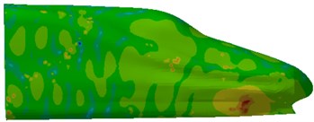
b) 300 Hz

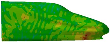
c) 500 Hz

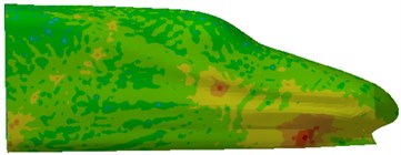
d) 700 Hz

5. Experimental verification of aerodynamic noises of the high-speed train

The computational model of the aerodynamic noise of the high speed train was relative complex, and it should be verified by the corresponding experiment. The experiment was conducted in a wind tunnel. The cross-sectional area was 8 m×6 m and the length was 15 m. The wind speed was controlled in 20 m/s-70 m/s. To reduce the influence of the floor boundary layer, the special floor for the train was mounted in the test section. A turntable with the diameter of 7 m and rotating range of 360° was placed in the middle of the floor, while other parts were fixed. The upper surface of the floor was 1.06 m away from the lower wind tunnel wall, and the center of the turntable was 7.84 m away from the front edge of the floor and 8.26 m away from the rear edge. The front and rear edges of the floor were processed to the streamlined shape to reduce the disturbance of airflow and inclined gaps between floors. Due to limitations of sizes of the wind tunnel, the scaling high-speed train was applied in the experimental process.

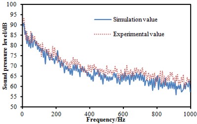
Three microphones were arranged in the head train to measure the sound pressure level of the observation point, as shown in Fig. 11. The measurement flow chart diagram was presented in Fig. 12. Bruel & Kjaer measurement instrumentation was used to collect the signal and then it was connected to the computer. The sampling frequency was 8000 Hz. The collected signal was processed by the Pulse software to obtain the sound pressure level. Each experiment was conducted three times to obtain the average value as the final result. Finally, the experimental result was compared with the simulation as shown in Fig. 13. It was indicated that the experimental SPLs were generally larger than the numerical simulation results mainly because the inflow in simulation process was set to be uniform flow, which could not be achieved in the experimental process. Besides, some details of the geometric model were cleared in the simulation process, thus resulting in some differences with the actual model. Finally, these factors would cause some errors which were within 5 dB, and errors can be accepted by the actual engineering. The prediction model can be considered effective.

Fig. 11Observation points and equipment

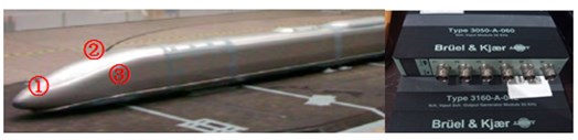
Fig. 12Experimental process of aerodynamic noises of the cabin

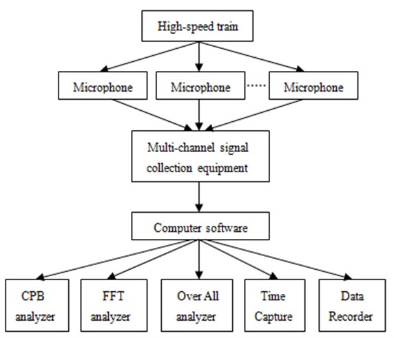
Fig. 13SPL comparison between experiment and simulation at three observation points

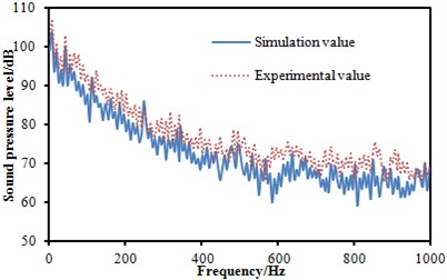
a) SPL comparison between experiment and simulation at observation point 1

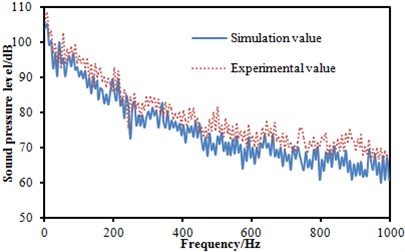
b) SPL comparison between experiment and simulation at observation point 2

c) SPL comparison between experiment and simulation at observation point 3

6. Conclusions

For improving noises in the cabin quickly, large eddy simulation was adopted to compute the fluctuating pressure of the cabin surface numerically. Then, the fluctuating pressure was mapped to the boundary element model as the excitation loads to obtain the aerodynamic noise distribution of the cabin at different frequencies, which was then compared with the experimental result. There were some differences between the computational model and actual model, and the experimental results were more than the simulation result, which was within the acceptable range of the engineering. The comparative result indicated that the prediction model was reliable. In addition, as presented from the computational results: SPLs on cabin surface were changed between 60 dB-110 dB, and greater SPLs were located on the transition position which was from the nose tip to the roof surface of the cabin. The aerodynamic noise on the cabin surface was mainly in low-frequency.

References

Shen Z. Y. Dynamic environment of high-speed train and its distinguished technology. Journal of the China Railway Society, Vol. 28, Issue 4, 2006, p. 1-5.

Search CrossRef
Goldstein M. V. Unified approach to aerodynamic sound generation in the presence of boundaries. Journal of the Acoustical Society of America, Vol. 56, Issue 2, 1974, p. 497-509.

Publisher
Kitagawa T., Nagakura K. Aerodynamic noise generated by Shin Kansen cars. Journal of Sound and Vibration, Vol. 231, Issue 5, 2000, p. 913-924.

Publisher
Sassa T., Sato T., Yatsui S. Numerical analysis of aerodynamic noise radiation from a high-speed train surface. Journal of Sound and Vibration, Vol. 247, Issue 3, 2001, p. 407-416.

Publisher
Nagakura K. Localization of aerodynamic noise sources of Shin Kansan trains. Journal of Sound and Vibration, Vol. 293, Issue 3, 2006, p. 547-556.

Publisher
Liu H. G., Lu S. L., Zeng F. L. Experimental study of automobile aerodynamic noise. China Journal of Highway and Transport, Vol. 18, Issue 1, 2005, p. 113-116.

Search CrossRef
Liu H. G., Lu S. L. Calculation method of the aerodynamic noise around high speed vehicles. Journal of Traffic and Transportation Engineering, Vol. 2, Issue 2, 2002, p. 41-44.

Search CrossRef
Liu J. L., Zhang J. Y., Zhang W. H. Numerical analysis on aerodynamic noise of the high-speed train head. Journal of the China Railway Society, Vol. 33, Issue 9, 2011, p. 19-26.

Search CrossRef
Xiao Y. G., Kang Z. C. Numerical prediction of aerodynamic noise radiated from high speed train head surface. Journal of Central South University, Vol. 39, Issue 6, 2008, p. 1267-1272.

Search CrossRef
Yuan L., Li R. X. Aerodynamic noise of high-speed train and its impact. Mechanical Engineering and Automation, Vol. 180, Issue 5, 2013, p. 31-35.

Search CrossRef
Yang Y., Yang G. W. A numerical study on aerodynamic noise sources of high-speed train. Proceedings of the 1st IWHIR, Vol. 2, 2012, p. 107-116.

Publisher
Sun Z. X., Song J. J., An Y. R. Numerical simulation of aerodynamic noise generated by CRH3 high speed trains. Acta Scientiarum Naturalium Universitatis Pekinensis, Vol. 48, Issue 5, 2012, p. 701-711.

Search CrossRef
Xiao Y. G., Tian H. Q., Zhang H. Prediction of interior aerodynamic noise of high-speed train cab. Journal of Traffic and Transportation Engineering, Vol. 8, Issue 3, 2008, p. 10-14.

Search CrossRef

About this article

Received

06 May 2016

Accepted

29 August 2016

Published

15 February 2017

SUBJECTS

Acoustics, noise control and engineering applications

DOI

https://doi.org/10.21595/jve.2016.17140

Keywords

high-speed trains

cabin

fluctuating pressure

aerodynamic noises

This is an open access article distributed under the Creative Commons Attribution License, which permits unrestricted use, distribution, and reproduction in any medium, provided the original work is properly cited.

Previous article in issue Previous Next article in issue Next

Research article

2018 02 15

Numerical simulation on the aerodynamic performance of the high-speed train under crosswinds

Ai Min Yang, Ce Zhang, Shan Shan Li, Ling Zhang, Xiao Jun Men, Fan Bei Kong, Shi Yu He

Research article

2017 08 15

Numerical computation and improvement of aerodynamic radiation noises of pantographs

Jin-mei Wu

Research article

2017 06 30

Numerical study on aerodynamic noises and characteristics of the high-speed train in the open air and tunnel environment

Xin Li, Tao Shang, Liu Han, Xiao-hong Jin, Li-hua Wang

Research article

2017 05 15

Numerical simulation of aerodynamic noises in the far field of the high-speed train with considering bogies and connection windshields

Wei-te Lu, Yan Wang, Chun-qin Zhang

M. Lv, D.- Xu, and H. He, “Numerical simulation and experimental study of aerodynamic noises for the cabin of the high-speed train,” Journal of Vibroengineering, Vol. 19, No. 1, pp. 678–689, Feb. 2017, https://doi.org/10.21595/jve.2016.17140

Copy Extrica

Copied to clipboard!

TY  - JOUR
DO  - 10.21595/jve.2016.17140
UR  - https://doi.org/10.21595/jve.2016.17140
TI  - Numerical simulation and experimental study of aerodynamic noises for the cabin of the high-speed train
T2  - Journal of Vibroengineering
AU  - Lv, Ming
AU  - Xu, Dong-er
AU  - He, Hua
PY  - 2017
DA  - 2017/02/15
PB  - JVE International Ltd.
SP  - 678-689
IS  - 1
VL  - 19
SN  - 1392-8716
ER  - 

Copy Ris

Copied to clipboard!

@article{Lv_2017,
	doi = {10.21595/jve.2016.17140},
	url = {https://doi.org/10.21595/jve.2016.17140},
	year = 2017,
	month = {feb},
	publisher = {{JVE} International Ltd.},
	volume = {19},
	number = {1},
	pages = {678--689},
	author = {Ming Lv and Dong-er Xu and Hua He},
	title = {Numerical simulation and experimental study of aerodynamic noises for the cabin of the high-speed train},
	journal = {Journal of Vibroengineering}
}

Copy Bibtex

Copied to clipboard!

[1]M. Lv, D. Xu, and H. He, “Numerical simulation and experimental study of aerodynamic noises for the cabin of the high-speed train,” Journal of Vibroengineering, vol. 19, no. 1, pp. 678–689, Feb. 2017, doi: 10.21595/jve.2016.17140.

Copy IEEE

Copied to clipboard!

Lv, Ming, Dong-er Xu, and Hua He. “Numerical Simulation and Experimental Study of Aerodynamic Noises for the Cabin of the High-Speed Train.” Journal of Vibroengineering 19, no. 1 (February 15, 2017): 678–89. https://doi.org/10.21595/jve.2016.17140.

Copy Chicago

Copied to clipboard!

Numerical simulation and experimental study of aerodynamic noises for the cabin of the high-speed train

Abstract

1. Introduction

2. Computational method of aerodynamic noises of the high-speed train

2.1. Main transmission process of aerodynamic noises

2.2. Control equations of large eddy simulation

2.3. Control equations of the acoustic boundary element method

3. Computation of aerodynamic characteristics of the high-speed train

4. Computation of aerodynamic noises of the high-speed train

5. Experimental verification of aerodynamic noises of the high-speed train

6. Conclusions

References

About this article

Related Articles