Discriminant analysis model of oil formation based on forecast probabilities of pressure changes

1. Introduction

It is well known that confidence intervals are a convenient and good criterion for the adequacy of the chosen model. However, confidence intervals can sometimes lead to incorrect results. Moreover, they cannot establish a difference between the candidate models of the formation, since the models are characterized by different sets of parameters with the corresponding dimensions of the probability distributions. As a result, it is difficult to compare different models in the space of parameters. This paper describes a new quantitative method for discriminant analysis of models, which allows to overcome these difficulties. This method is a direct continuation of the methods for obtaining confidence intervals based on Bayesian inference. The idea of the method is that the correct model should more accurately predict the pressure changes than other models. From a quantitative point of view, the probability of a real change in pressure at future times for a correct model should be higher than the predicted probability for the remaining models. The predicted probability distribution of events associated with pressure changes can be calculated with known probability distributions of the parameters. Similar to the proposed approach, the methods are discussed in [1].

2. The structure of the algorithm

The basic algorithm of the method of sequential probability prediction (MSPP) for the discriminant analysis of reservoir models based on well test is as follows.

1) Select several candidate reservoir models that, in one way or another, are consistent with well test and other available information.

2) Use the first few results of pressure measurement to evaluate the reservoir parameters and predict the probability distribution for pressure at the next time point for each reservoir model.

3) Calculate the probability by substituting the actual pressure values in the formula for the predicted probability distribution and update the value of the total probability by multiplying it by the calculated probability with respect to each reservoir model.

4) Repeat the steps until a difference in the total probabilities for each reservoir model is achieved.

5) Discriminant analysis of reservoir model candidates is carried out based on the calculated total probabilities.

3. The mathematical model

The condition that the function describing the model can be approximated by expanding it in a Taylor series of the first order leads to the following expression:

where $\mathbf{\theta }$ – a vector of $m$ of unknown parameters of layer, $\widehat{\mathbf{\theta }}$ – the average (expected) values of parameters (an assessment of $\mathbf{\theta }$ by a method of the smallest squares on the basis of $n$ of independent observations).

The predicted probability distribution for each model is determined in accordance with the following procedure in the Bayesian derivation. In this case, the parameters $\mathbf{\theta }$ are considered random variables with some probability distributions.

Suppose that we know the variance ${\sigma }^2$ of these distributions. Then the uncertainty associated with the model is described by the equation [2, 3]:

where $y_i$ is the pressure value for $i$ observation, $\mathbf{H}$ is the Hessian matrix in the Gauss method [4]:

In this case, the parameters $\mathbf{\theta }$ form a multidimensional normal distribution around $\widehat{\mathbf{\theta }}$ with the covariance matrix ${\sigma }^2{\mathbf{H}}^{-1}$ with known $n$ independent observations of the pressure measurement results. $\mathbf{\theta }$ is a dimension vector $m$, and hence their probability distribution also has the dimension $m$.

Using the $\widehat{\theta }$ and $n$ parameter estimates, the real pressure value $y_{n+1}^{*}$ at the $x_{n+1}$ point is expressed by Taylor expansion with the terms up to the first order:

The gradient of the model function $\mathbf{g}$ is calculated at the $x_{n+1}$ point using the estimated values of the parameters based on the first $n$ observations.

Having chosen the notation ${\widehat{y}}_{n+1}=F\left(\widehat{\mathbf{\theta }},x_{n+1}\right)$, Eq. (4) can be represented in the form:

In accordance with Eq. (2), $y_{n+1}^{*}$ is normally distributed relative to ${\widehat{y}}_{n+1}$ with the predicted variance:

and conditional probability:

Eq. (8) characterizes the uncertainty associated with the model, which shows how adequate it is, and is completely determined by the average (expected) value of ${\widehat{y}}_{n+1}$ and the forecast variance ${\sigma }_p^2$.

The projected variance ${\sigma }_p^2$ affects three important points. First, Eq. (7) shows that the forecast variance contains all information about the uncertainty concerning the parameters, since It is calculated using the covariance matrix ${\sigma }^2{\mathbf{H}}^{-1}$. Second, it follows from the Schwartz inequality that the value of the predicted variance is limited by the determinant of the matrix ${\sigma }^2{\mathbf{H}}^{-1}$:

The more information about the parameters received, the lower the uncertainty associated with them. The dimension of the multidimensional normal distribution becomes narrower, and the determinant of the covariance matrix decreases. Accordingly, the forecasted variance decreases. Therefore, when the multidimensional normal distribution for the parameters takes the form of the Dirac delta function [2], the normal distribution for the true pressure change relative to the predicted (expected) pressure change also narrows to the delta function. In other words, the uncertainty associated with the parameters is transformed into an uncertainty associated with a change in pressure. And, finally, more importantly, the predicted variance is a scalar quantity regardless of the dimensionality of the covariance matrix. Thus, models with a different number of parameters can be compared using predictive variance.

Fig. 1The relationship between Probyn+1*y^n+1, Probyn+1yn+1* and Probyn+1y^n+1

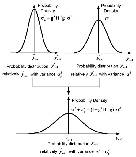
The uncertainty associated with the data is described as follows. Suppose that the observed change in pressure $y_{n+1}$ is normally distributed relative to the real pressure change $y_{n+1}^{\mathrm{*}}$ with the variance ${\sigma }^2$:

Exactly the same assumption was made in the derivation of Eq. (2). Eq. (10) expresses the uncertainty associated with the data, which characterizes how well the model corresponds to the data.

Since the exact value of $y_{n+1}^{\mathrm{*}}$ is unknown, the relationship between $y_{n+1}$ and ${\widehat{y}}_{n+1}$ is set by an exception in the integration by $y_{n+1}^{\mathrm{*}}$:

As a result, the observed pressure change $y_{n+1}$ is normally distributed with respect to the predicted (expected) pressure change $y_{n+1}^{\mathrm{*}}$ with the overall predicted variance ${\sigma }^2+{\sigma }_p^2=\left(1+{\mathbf{g}}^T{\mathbf{H}}^{-1}\mathbf{g}\right)\cdot {\sigma }^2$. This variance links the uncertainty of the ${\sigma }_p^2$ model and the uncertainty in the ${\sigma }^2$ data, as shown in Fig. 1.

4. Numerical simulations and results

The result of substituting the observed pressure change $y_{n+1}$ in Eq. (11) is the probability of observing $y_{n+1}$ at the moment $x_{n+1}$ for this model based on the first observations. This procedure is schematically shown in Fig. 2. Here the $x$ axis corresponds to the time, and the $y$ axis to the pressure.

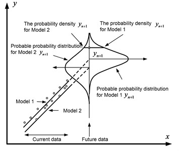
In Fig. 3 presents the probable probability distributions for the two models, which are designated as Model 1 and Model 2. It is seen that the probability of $y_{n+1}$ for the first model is higher than for the second. Therefore, Model 1 is more adequate than Model 2.

Fig. 2Schematic representation of the method of forecasting probabilities

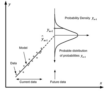
Fig. 3Schematic representation of the probability prediction method for two models

Eq. (11) indicates that the probability of observing $y_{n+1}$ at the moment $x_{n+1}$ will be the higher, the smaller the total predicted variance ${\sigma }^2+{\sigma }_p^2$ and the observed change in pressure $y_{n+1}$ closer to the predicted (expected) value of ${\widehat{y}}_{n+1}$.

In Fig. 4 shows three possible cases for the two models. So, in Fig. 4(a), the expected pressure changes for the two models coincide, and the total predicted variances differ. In this case, the probability of observing $y_{n+1}$ for a model with a smaller variance will be higher. In Fig. 4(b), the expected pressure changes for the two models are different, and the overall predicted variances are the same. In this case, the probability of observing $y_{n+1}$ will be higher for a model in which the expected change in pressure is closer to its actual value. In Fig. 4(c) the expected pressure changes and the overall predicted variances differ. Then the probability of observing $y$ will be higher for a model that has a smaller variance and whose expected change in pressure is closer to its actual value.

Fig. 4Three possible cases of predictive probability distributions for two models

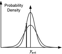
a) The same expected values, different variances

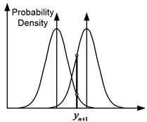
b) Different expected values, identical variances

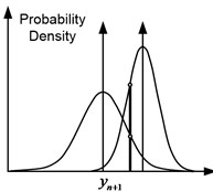
c) Different expected values, different variances

However, in cases where the actual change in pressure is closer to the expected value for a model with a larger overall predictive variance, this model will have a higher probability of observing $y_{n+1}$ at the time of $x_{n+1}$. This suggests that this model, which has a large overall predictive variance at this stage, may prove to be a correct model in the future. That is, a sequential procedure is used to check whether this assumption is true [5].

In other words, substituting the actual pressure change in the formula for the predicted probability distribution for each model is the process of deciding which of the models is most appropriate at the current stage. In this case, the sequential procedure is the accumulation of the results of decision-making at all stages.

In the case when the variance ${\sigma }^2$ is unknown, instead of Eq. (2) it is necessary to use equation:

Then Eq. (11) will be transformed to the form:

Thus, when the variance ${\sigma }^2$ is unknown, $y_{n+1}$ forms an $t$ – distribution relative to ${\widehat{y}}_{n+1}$ with a total predictive variance of $s^2+s_p^2=\left(1+{\mathbf{g}}^T{\mathbf{H}}^{-1}\mathbf{g}\right)s^2$ and $n-m$ degrees of freedom.

It should be noted that as the $n$ increases, the $t$ distribution becomes normal. Moreover, with $n-m\ge 30$ instead of $t$ – distribution, it is entirely possible to use the corresponding normal distribution.

The projected variance plays a key role in MSPP. Typically, ${\mathbf{g}}^T{\mathbf{H}}^{-1}\mathbf{g}$ is smaller for a simpler model. To verify this, the probabilistic probability was studied for several reservoir models [6, 7]:

– radial flow in an infinite formation (three parameters: $k$, $S$ and $C$);

– with a non-conductive reset (four parameters: $k$, $S$, $C$ and $r_e$);

– with an impenetrable outer boundary (four parameters: $k$, $S$, $C$ and $r_e$);

– with constant pressure at the external boundary (four parameters: $k$, $S$, $C$ and $r_e$);

– with double porosity and pseudo-stationary inter-porous flow (five parameters: $k$, $S$, $C$, $\omega$ and $\lambda$);

– with double porosity, pseudo-stationary inter-porous flow and non-conductive reset (six parameters: $k$, $S$, $C$, $\omega$, $\lambda$ and $r_e$);

– with double porosity, pseudo-stationary inter-porous flow and impermeable outer boundary (six parameters: $k$, $S$, $C$, $\omega$, $\lambda$ and $r_e$);

– with double porosity, pseudo-stationary inter-porous flow and constant pressure at the outer boundary (six parameters: $k$, $S$, $C$, $\omega$, $\lambda$ and $r_e$).

We studied the predictive probability characteristics for radial flow models in an infinite reservoir, a reservoir with a non-conductive discharge, a reservoir with an impenetrable outer boundary, and a reservoir with constant pressure at the outer boundary. From the point of view of the number of parameters, the flow model in an infinite reservoir was considered as a simple model, the rest as complex. In Fig. 5 shows the typical pressure variation curves and the corresponding ${\mathbf{g}}^T{\mathbf{H}}^{-1}\mathbf{g}$ values. Information on the formation and fluid: borehole radius $r_w=$0.1 m, reservoir thickness $h=$5 m, volume factor $B_o=$1 [m³]reservoir/[m³]norm , viscosity $\mu =$10^-3 Pa·sec, porosity $\varphi =$0.2, initial pressure $P_i=$20 MPa, total compressibility $c_t=$ 10^-4 MPa^-1, operating rate $q=$100 m³/day. The true values of the parameters are $k=\mathrm{}$0.05 µm², $S=\text{10}$ and $C=\mathrm{}$0.2 m³/MPa. For reservoir models with a $r_e=$ 600 m boundary. Pressure data was used without adding random errors. The total number of data points was 101. The Hesse inverse ${\mathbf{H}}^{-1}$ matrix was calculated using points at the moments from $x_1$ to $x_n$. The gradient $\mathbf{g}$ was determined at the $x_{n+1}$ point. $n$ changed from 41 to 100. The effect of the boundary is already noticeable from the moment of $x_{67}\approx$ 20 h. In Fig. 5b oscillations in the values of ${\mathbf{g}}^T{\mathbf{H}}^{-1}\mathbf{g}$ for complex models are noticeable due to rejection errors caused by the applied method of numerical inverse Laplace transform. With the exception of the reservoir model with constant pressure at the outer boundary, the values of ${\mathbf{g}}^T{\mathbf{H}}^{-1}\mathbf{g}$ for the other complex models are always higher than for the simple model (the radial flow model in an infinite reservoir). Due to the boundary effects, the values of ${\mathbf{g}}^T{\mathbf{H}}^{-1}\mathbf{g}$ for the reservoir model with constant pressure at the outer boundary become less than ${\mathbf{g}}^T{\mathbf{H}}^{-1}\mathbf{g}$ for the radial flow model in the infinite formation.

Fig. 5The first study of predictive variance

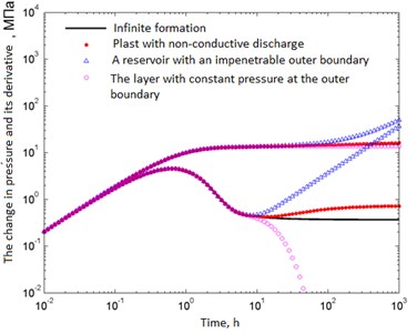
a)

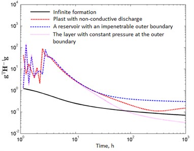
b)

5. Conclusion

On the basis of Fig. 5, we can conclude that for typical pressure variation curves the value decreases in the direction of simplification of the model.

The developed method provides a universal tool for discriminant analysis of models regardless of the number of parameters used. In this respect, the method compares favorably with methods based on confidence intervals, which cannot be used to compare models with different sets of unknown parameters. For example, it is not possible to directly compare the confidence intervals of permeability for two different models, such as the flow model in an infinite reservoir with three parameters ($k,s,C$) and the non-conductive four-parameter reservoir model ($k,s,C,r_e$), because in the latter model, a strong negative correlation exists between $k$ and $r_e$.

The method takes into account not only the diagonal elements of the inverse Hessian matrix, but also the elements outside the main diagonal, and therefore it uses all available information about the parameters by means of the predictive variance. It should be noted that methods based on confidence intervals take into account only the diagonal elements of the Hessian matrix.

This method meets the requirements of both the simplicity and complexity of the model. Theoretically, with an increase in the number of parameters, the overall correspondence of the model to the initial data increases due to a decrease in the number of degrees of freedom. However, the complication of the model reduces its predictable efficiency. This relationship is expressed quantitatively through ${\sigma }^2$ and ${\mathbf{g}}^T{\mathbf{H}}^{-1}\mathbf{g}$, which are components of the uncertainty associated with the model (${\mathbf{g}}^T{\mathbf{H}}^{-1}\mathbf{g}\cdot {\sigma }^2$). In general, ${\sigma }^2$ it decreases with increasing complexity of the model, whereas ${\mathbf{g}}^T{\mathbf{H}}^{-1}\mathbf{g}$ decreases with the simplification of the model. In this case, the overall forecast variance ${\sigma }^2+{\sigma }_p^2=\left(1+{\mathbf{g}}^T{\mathbf{H}}^{-1}\mathbf{g}\right)\cdot {\sigma }^2$ takes into account both the simplicity and the complexity of the model.

The proposed method can simultaneously compare any number of reservoir models. Moreover, it is not required that any of the models be a subset of the other.