Processing curves pressure changes on the results of well test based on fuzzy regression trees

1. Introduction

Mathematical models of the reservoir-reservoir are created by solving the diffusion equation under various boundary conditions. Models are defined by three different components that characterize the formation, the well and its vicinity (internal boundary conditions) and the outer boundaries of the formation (external boundary conditions). In the general case, the change in pressure is first due to the influence of internal boundaries, then at intermediate times the pressure change corresponds to the basic behavior of the productive formation, and finally, after a sufficiently long time, the pressure change is determined mainly by external boundary conditions.

The general equation of fluid filtration in an oil reservoir is described by the following diffusion equation [1]:

where $P$ is the pressure; $r$ – distance along the radius from the wellbore; $t$ – time; $\varphi$ – porosity; $\mu$ – viscosity; $c_t$ – the total compressibility of the system; $k$ – absolute permeability.

To obtain analytical solutions of the diffusion Eq. (1), the Laplace integral transformation is applied, which leads to a smoothing of the errors of the experimental functions. In addition, based on the exact solution in images, it is possible to obtain asymptotic solutions for $t\to \mathrm{\infty }$ and $t\to 0$ in the time domain and to use them effectively in solving inverse problems [4].

One way or another, the application of the Laplace transform is limited to those cases when the solution of the differential equation can be obtained analytically. However, this is not always the case. Therefore, if an exact solution cannot be obtained, it is possible to replace the differential equation by its finite-difference analogue [4, 5]. The definition of the parameters of linear and nonlinear differential equations refers to the construction of the so-called “gray box” model. The model is called so, since its mathematical structure is given in explicit form. The relationships between all parameters and variables of the model are known. The gray box model is convenient for using various methods of system identification.

2. Computational example

Let us consider an example of a simple model of heat propagation in an isolated metal rod of length $L$ [3]. One end of the rod is heated with thermal power $u\left(t\right)$, at the other end a temperature measurement is performed $y\left(t\right)$. Under ideal conditions, this system is described by the equation of thermal conductivity (diffusion):

where $\kappa$ is the coefficient of thermal conductivity; $x\left(t,\xi \right)$ – rod temperature at point $\xi$ at the time $t$.

To obtain a time-continuous model in the state space, the second derivative on the right-hand side of Eq. (2) is replaced by a finite-difference approximation:

where $\xi =k\mathrm{\Delta }L$; $k=\mathrm{1,2},\dots ,n$; $n=L/\mathrm{\Delta }L$. Such a transformation leads to a system with a finite set of $n$ states $x\left(t,k\mathrm{\Delta }L\right)$, Each of which represents a certain average temperature of the rod in the range $k\mathrm{\Delta }L\le \xi <\left(k+1\right)\mathrm{\Delta }L$. In other words, the order of the system depends on the size $\mathrm{\Delta }L$ of the spatial grid.

As a result, the diffusion Eq. (1) can be represented as a time-continuous linear system in the state space:

where $\mathbf{x}\left(t\right)$ is the state vector; $\mathbf{u}\left(t\right)$ – input vector; $\mathbf{e}\left(t\right)$ – vector of noises; $\mathbf{y}\left(t\right)$ – system reaction vector; ${\mathbf{x}}_0$ – vector of initial states of the system. For our problem:

Furthermore, having sufficient observations can use any suitable method for identification systems (e.g., a method of minimizing the prediction error (PEM), which is largely based on an autoregressive moving average model, taking into account external influences (ARMAX) for estimating parameter $\kappa$.

3. The derivation of the scheme

Despite the great flexibility of the described method of replacing a differential equation by a finite-difference one, it has a number of serious drawbacks. This approach should be applied with great caution, since finite-difference approximation is equivalent to direct differentiation of experimental functions and is fraught with large errors [4, 5]. In addition, there is, for example, a reservoir model with a non-conductive discharge, which, in fact, is two-dimensional. If we use the Laplace transform, then for this model there is an analytical expression for changing the pressure in the well. However, the use of a numerical solution of this problem for obtaining system Eq. (4) may require an excessive number of state variables. Also, it may be noted that there are certain difficulties in creating a model of the form Eg. (4) for processing well test data obtained pressure recovery method. The problem is related to the dependence of the vector of initial conditions on the parameters of the formation.

In addition to the difficulties mentioned above, when working with finite differences, there is perhaps the main obstacle to the wider application of models of the type Eq. (4). For each new set of observations, the corresponding differential equation must be solved each time, which is associated with a large computational cost. It would be more convenient to have in advance a set of numerical solutions that would approximate the complex functional relationship between the independent variables (in this case the flow rate of the well), the parameters (in this case the formation) and the dependent variables (in this case the well pressure). For such purposes, so-called soft computing methods are widely used: neural networks and fuzzy logic inference systems [2]. As shown by a number of studies [1], the latter are usually preferable. The reasons are more simple adjustment of fuzzy systems, as well as a more understandable internal structure and logic of the operation of such systems, based on rules.

Modern systems of fuzzy inference are based on the application of a particular method of structural optimization to determine the structure of its rules base [8]. To solve the problems of non-linear regression, the classification and regression tree (CART) trees, which are special cases of decision trees, have gained particular popularity. With minor changes, CART can be used to identify the structure of the fuzzy rules base. Consider the basic steps necessary to generate a fuzzy logic inference system based on CART as applied to the analysis of well data.

The well test method of pressure recovery was formed on the basis of the analytical model:

where $P_{D_{BU}}$ – dimensionless pressure change in well test method of pressure recovery; $P_D$ – dimensionless pressure change during well testing by lowering the level; $t_D$ – dimensionless time change; $t_{pD}$ – dimensionless time during which production was carried out prior to the closure of the well.

Information on the reservoir and the fluid that saturates it is taken from Table. 1. The total number of points $N_t$ over a period of 0.01 to 100 hours was 51. In general, $N_c=\text{50}$ random pressure curves were generated. Half of them were used as a training sample, the other half as a test sample. In this case, the areas of changes in the parameters $k$, $S$ and $C$ were, respectively $\left[\mathrm{0,01};\mathrm{0,1}\right]$ µm², $\left[0;10\right]$ and $\left[\mathrm{0,01};\mathrm{0,1}\right]$ m³/MPa. The total volume of observation points $N_s=N_t{N}_c=\text{2550}$.

In view of the wide variation in the values of time and the change in pressure, instead of real values $t$ and $\mathrm{\Delta }{P}_{BU}$ during training, we used, respectively $\mathrm{l}\mathrm{o}\mathrm{g}\left(t\right)$ and $\mathrm{l}\mathrm{o}\mathrm{g}\left(\mathrm{\Delta }{P}_{BU}\right)$. This has positively affected the entire learning process, so it is known that correct scaling of dependent and independent variables can significantly improve the conditionality of the problem [7].

In accordance with the CART algorithm, a regression tree was constructed to predict the response $\mathrm{\Delta }{P}_{BU}$ as a function of the predictors $k$, $S$, $C$ and $t$.

In the work, the fuzzy system performed a logical conclusion by Sugeno (in particular, the fuzzy first-order Sugeno model is used), since this simplifies the further parametric adjustment of the system [10, 12].

Since the regression tree is a particular case of a decision tree, it can be represented as a set of clear rules. Denote the set of independent variables and parameters at the input of the tree as $\left\{\left.x_i\right|i=\overline{1,I}\right\}$ and the dependent variable at the output of the tree as $y$. Any rule consists of a premise and a corollary. The premise in this case is the result of a comparison $x_i$ with a certain threshold value $w_n$ in the $n$-th node of the tree ($n=\overline{1,N}$). Let $v_n\in \overline{1,I}$ be the index of the input variable, by which the comparison takes place in the $n$-th node of the tree. Each tree node, except terminal nodes (leaves), has two descendants: left and right. If the result $x_{v_n}<w_n$ is true, further comparisons are made in the left child node. If the result $x_{v_n}\ge w_n$ is true, further comparisons are performed in the right child node. In the future, without specifying the type of relationship, we will write down simply $x_{v_n}\circ w_n$. Then any rule can be represented in the following general form:

where $m\in \overline{1,N}$ – the index of the node, only through which it is possible to get into the $l$-th sheet.

In order to make the clear rule Eq. (6) unclear, it is necessary to fuzzy the premises and the consequence of the rule. In the premise $x_{v_n}\circ w_n$ is replaced by the operation of belonging to a fuzzy set ${\mathcal{A}}_n$, i.e. $x_{v_n}\in {\mathcal{A}}_n$. This is equivalent to calculating the membership function ${\mu }_{{\mathcal{A}}_n}\left(x_{v_n}\right)$, in which the sigmoid function was chosen:

where usually $c_n=w_n$; ${\alpha }_n$ is configured by the user or calculated automatically. Moreover, the sign determines the type of fuzzy relation.

During the construction of the tree, a training sample was used, which can be represented as an ordered set of observations $\mathcal{S}=\left\{\left.\left(x_{1,d},\dots ,x_{I,d},y_d\right)\right|d=\overline{1,D}\right\}$. When a tree is traversed, each q-th node, including the terminal one, can be assigned a subset ${\mathcal{S}}_q\subset \mathcal{S}$ as a result of the decomposition ${\mathcal{S}}_n\subseteq \mathcal{S}$ for $n$-th node, who is the parent of the $q$-th node. The breakdown is carried out in accordance with $x_{v_n}\circ w_n\text{.}$ In this case, the equalities ${\stackrel{-}{x}}_n=\frac{1}{D_n}\sum _{d=1}^{D_n}{x}_{v_n,d}$ and $y_l=\frac{1}{D_l}\sum _{d=1}^{D_l}{y}_d.$

Let us calculate the following mean square error:

As a result, the parameter ${\alpha }_n$ in Eq. (7) can be associated with ${\sigma }_n$ the following way:

where $\mathrm{e}\mathrm{r}\mathrm{f}\left(x\right)$ – error function; $K>0$.

The choice ${\alpha }_n$ of Eq. (9) ensures equality of the areas under $\mathrm{s}\mathrm{i}\mathrm{g}\left(x;{\alpha }_n,c_n\right)$ and the Laplace function $\mathrm{\Phi }\left(x;c_n,{\sigma }_n\right)$ in the interval $\left[-K{\sigma }_n;K{\sigma }_n\right]$. Experiments have shown that the choice $K=1$ is quite satisfactory.

A consequence in the fuzzy Sugeno rule is presented in the following form [10, 12]:

Let us denote ${\mathbf{X}}_l={\left[x_{i,d}\right]}^T$ the matrix of observations of input variables that fall into the $l$-th sheet, and ${\mathbf{y}}_l=\left[y_d\right]$ is the vector of observations of the output variable in the same sheet. Then, to find the vector of unknown parameters ${\mathbf{p}}_l=\left[p_{m,l}\right]$, $m=\overline{0,I}$ we need to solve the following normal equations:

where ${\tilde{\mathbf{X}}}_r=\left[\left.{\mathbf{X}}_r\right|1\right]$ – supplemented by units to the right of the matrix of input observations.

The solution Eq. (11) can be carried out by any suitable factorization method of the matrix ${\tilde{\mathbf{X}}}_r$. If ${\tilde{\mathbf{X}}}_r$ turns out to be degenerate, then we can use the Sugeno model of zero order:

Fig. 1Mean square error in training and test samples

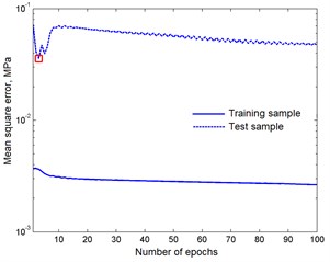
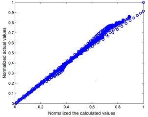
Fig. 2Cross-raft of normalized actual and calculated values

4. Results and discussions

After the structure of the fuzzy system has been determined, its parametric adjustment (optimization) [6, 9] is required, at which both the rule conclusions and the membership functions of the terms of the input variables are adjusted at the same time. The hybrid optimization method ANFIS [8, 11] (adaptive neural-fuzzy inference system), in which the linear parameters are tuned for the Kalman filter, and the non-linear parameters by the gradient method of back propagation of the error, proved particularly successful. However, in principle, all parameters can be adjusted only by the gradient method, that is, like the neural network training algorithms.

In the study, the tuning was performed on the basis of ANFIS using the same training sample as in the construction of CART. To avoid retraining the fuzzy system, a test sample was tested at this stage. In Fig. 1 shows the graphs of mean-square errors obtained from the training and test samples. A square is marked by a fuzzy system having a minimum error on the test set. In Fig. 2 a cross-raft is constructed, where the normalized values produced by the fuzzy system are located along the abscissa axis and the normalized values from the test sample along the ordinate. Correlation coefficient $\rho =\text{0,9968}$.

To simulate the random error, normally distributed, the data well testing used a random number generator with zero expectation and variance 10-4 МPа². The true values of the parameters were $k=$ 0,05 mkm², $S=\text{5}$, $C=$ 0,05 m³/MPа.

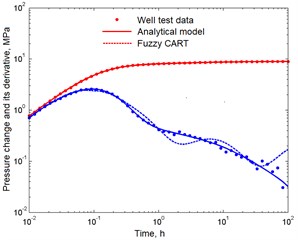
The results of parameter estimates using the analytical model and fuzzy CART are given in Table 2. The curves of the change in pressure and its derivative obtained by both methods are shown in Fig. 3.

Fig. 3Dynamics of pressure and its derivative

5. Conclusions

Based on the studies carried out, the following conclusions can be drawn. Fuzzy systems, whose structure of rules base are formed on the basis of CART, are really capable of approximating complex nonlinear dependencies between independent variables, parameters and dependent variables. Such systems can be successfully used to perform nonlinear regression analysis. However, they should not expect high accuracy, the resulting estimates, as in the case of analytical or numerical models. The main application of fuzzy inference systems is seen in distinguishing between candidate models.