A method for shifting natural frequencies of a dynamic system to desired values with concentrated mass modifications

1. Introduction

Shifting the natural frequency of a system is an important issue in the structural modification. This may be made for avoiding resonance or fitting the numerical models to the experimental models. The main challenge is the determination of necessary modifications for shifting the natural frequencies to the desired values. This problem has been studied by many researchers for a long time. Although the problem was well defined, the researchers have been interested in developing the efficient methods. Tsuei and Yee [1] presented a method for the determination of necessary modifications to shift the natural frequencies of a dynamic system to desired values. The method is iterative and uses the forces responses of the system. Bucher and Braun [2] developed a theory to show how the necessary mass and stiffness modifications can be computed using only the modal test results, even when only a partial set of eigen-solutions is available from the tests. Ram [3] presented a strategy for enlarging a spectral gap by adding two appropriate oscillators at the proper locations. McMillan and Keane [4] studied shifting resonance from a frequency band applying concentrated masses to a plate. Sivan and Ram [5] developed a method for determining mass and stiffness modifications to achieve desired natural frequencies by using modal analysis. The difficulties arising from truncated data provided by modal analysis were overcome by an optimization procedure. Chang and Park [6] proposed a method based on frequency response function (FRF) sensitivity analysis for modal updating. The suggested method was applied to estimation of spring stiffness values in a spring supported plate. Li and He [7] proposed a method based upon use of FRF data in order to determine mass and stiffness modifications of an undamped structural system that are needed to change the dynamic characteristics of the system. Their approach formulates the structural modification problem using a set of linear equations. Park and Park [8] proposed some methods based on FRF based-substructure-coupling concept for the identification of structural parameters. Mottershead and his coworkers [9-13] presented a series of papers on assigning poles and zeros to the dynamical systems. Farahani and Bahai [14] proposed an inverse strategy for the relocation of natural frequencies. In the proposed method, a sensitivity analysis of the system’s eigenvalues, with respect to material or geometrical parameters of the structure, was conducted. The required parameter variation to achieve a desired frequency shift for the structure was then computed. Lawther [15] presented a comprehensive study on removing frequencies from a given range by changing the stiffness. The success of the method was assessed according to both the rank of changes and the number of freedoms that they connect to. Recently, Ouyang and his coworkers [16-19] have studied the passive structural modifications of the mass-spring systems for assignment of the eigen-structures i.e. eigen-values and eigen-vectors. The proposed methods are based on the use of modal parameters, physical properties or response properties and the problem is solved by sensitivity analysis, iterations or optimisation. The physical modifications may be in the form of mass, stiffness and damping. Sometimes a mass-spring system is added to the original system such that this introduces an additional degree of freedom. Although, the existing methods mentioned above has its own advantages and disadvantages, it can be concluded that the methods use FRFs are more suitable for the practical applications. Because FRFs are directly measured on the test structure. On the other hand, the mass modification is the simplest modification type which can easily be applied in practice. Also, this type of modification does not introduce additional degree of freedom to the original system. In this respect, the motivation of this paper can be clarified as follows: to develop a method for shifting the natural frequencies of a system to the desired values by the mass modifications, which uses measured FRFs of the original system without needing the physical or modal parameters; to advance Sherman-Morrison (SM) formula [20], for the inverse structural modification aim, which is successfully used for the solution of various structural modification problems in the past.

In this study, a new method is proposed in order to shift a certain number of prespecified resonance frequencies of the dynamic systems to desired values by adding concentrated masses. The method is based on the Sherman-Morrison formula and it estimates the necessary mass modifications by solving a certain number of non-linear equations which equal the number of necessary modifications. The method uses a number of receptances related to the modification coordinates of the original system and does not need the physical or modal properties. The numerical simulations, as well as the experimental studies made on a steel beam, show the efficiency of the proposed method.

In the next section, the structural modification method based on the SM formula is presented first. Then the method developed for the determination of the necessary mass modifications is introduced. After the verification of the method by numerical simulations, an experimental application is also given. Lastly, the results of the proposed method are concluded.

2. Theory of structural modification based on the SM formula

The method proposed here is based on the SM formula [20] that allows one to compute the inverse of a modified matrix by using the inverse of the original matrix and the modification. The structural modification based on the SM formula was well defined as follows [21-24]:

where [${\alpha }^{*}$] and [$\alpha$] are the symmetric receptance matrices of the modified and the original systems, respectively. The vectors $\left\{u\right\}$ and $\left\{v\right\}$ consist of the modifications. If a mass $\delta m$ is added to the system at coordinate $r$, then the $r$th elements of $\left\{u\right\}$ and $\left\{v\right\}$ are $u_r=$1, $v_r=-{\omega }^2\delta m$, respectively and the other elements are zero.

Although all the elements of the receptance matrix [$\alpha$] of a test structure are needed in Eq. (1), it can be written at active coordinates only, i.e., response, excitation and modification coordinates [22]. Furthermore, in the case of more than one modifications it can be sequentially applied. In this respect, if $n$ mass modifications $\delta m_i$ ($i=$1, 2,…, $n$) are made on a structure, the receptances of the modified system relating the active coordinates can be calculated sequentially as follows:

where the matrices and the vectors are written in bold characters for convenience, the superscript $a$ shows the active coordinates, $i$ is the modification step, and $\omega$ is the angular frequency in rad/s. The elements of ${\mathbf{u}}_i$ and ${\mathbf{v}}_i$ corresponding to the modification coordinates are one and the others are zero.

3. Method for the determination of the necessary mass modifications

The aim of this study is the shifting of a certain number of natural frequencies to desired values with mass modifications. For the calculation of necessary mass modifications, a method, which uses Eq. (2) in an inverse manner, is proposed. In order to clarify the method proposed, first the single natural frequency case is considered. It is required that the system has a natural frequency at ${\omega }_{s1}$ after a mass modification. In this case the receptance value of the modified system at ${\omega }_{s1}$ goes to infinity for an undamped system. This means that the denominator of Eq. (2) is zero at ${\omega }_{s1}$. In this way, equating the denominator of Eq. (1) to zero for $n=i=$1, one can obtain:

where ${\mathbf{\alpha }}_a^0$ is the receptance matrix of the original system related to the active coordinates. For the single mass modification at coordinate $r$, all of the elements of vectors $\mathbf{u}$ and $\mathbf{v}$ are zero except the modification coordinate, Eq. (3) yields:

and consequently, the necessary mass modification can easily be found from the Eq. (4) as follows:

where ${\alpha }_{rr}^0\left({\omega }_{s1}\right)$ is the receptance value of the original system, corresponding to the modification coordinate $r$, at frequency ${\omega }_{s1}$. It should be noted that Eq. (5) is precise and it is not surprising that it is similar to what was given in [7, 13].

In order to generalize the method for shifting $n$ frequencies, consider two natural frequencies of the system that are shifted to ${\omega }_{s1}$ and ${\omega }_{s2}$ by modifying the system with two masses at two prespecified coordinates. Two mass modifications $\delta m_1$ and $\delta m_2$ can be made by using Eq. (2), sequentially. By this way, for $n=$2 and $i=$1, 2, the receptance matrix of the modified system for each step can be written as:

where ${\mathbf{\alpha }}_a^1$ is the recepatance matrix of the system modified with mass $\delta m_1$, and ${\mathbf{\alpha }}_a^2$ is the recepatance matrix of the final system which is modified with both masses $\delta m_1$ and $\delta m_2$. For the final system has two natural frequencies at ${\omega }_{s1}$ and ${\omega }_{s2}$, the denominator of Eq. (7) is equated to zero at these frequencies. By assuming the modifications $\delta m_1$ and $\delta m_2$ are made at coordinate $p$ and $r$, respectively, then the elements of vectors ${\mathbf{u}}_1$ and ${\mathbf{v}}_1$ corresponding to the coordinate $p$ in Eq. (6) and the elements of vectors ${\mathbf{u}}_2$ and ${\mathbf{v}}_2$ corresponding to the coordinate $r$ in Eq. (7) are one and all of the others elements are zero. Consequently, this yields two nonlinear equations with two unknowns as follows:

where ${\alpha }_{rr}^1\left({\omega }_{si}\right)$; $i=$ 1, 2 can be determined by means of Eq. (6) as follows:

By substituting Eq. (9) into Eq. (8) and solving the derived equations numerically the necessary mass modifications can be obtained. It is clear that this approach can easily be extended for the shifting of more than two frequencies in a similar way. For shifting $n$ natural frequencies to the desired values, if the last modification is assumed to be at the coordinate $q$, then $n$ nonlinear equations with $n$ unknown masses can be written as follows:

where ${\alpha }_{qq}^{n-1}\left({\omega }_{si}\right)$, ($i=$1, 2,..., $n$) are determined sequentially, similar to method in Eq. (9), then the unknown mass modifications $\delta m_i$, ($i=$1, 2,..., $n$) can be estimated by solving the equation set Eq. (10) numerically.

The proposed method for the general case can be applied as follows: (i) The desired natural frequencies and the modification locations are chosen. (ii) The FRFs related to the modification locations are measured. If the measured FRFs are the accelerance or the mobility they have to be transformed to the receptance for the next calculations. (iii) The FRFs of the modified system are sequentially determined by means of Eq. (2). Note that; it is clear from Eq. (2) that the FRFs of the modified system can be determined symbolically; due to $\delta m_i$, ($i=$1, 2,..., $n$) is unknown. (iv) The necessary mass modifications are estimated by solving Eq. (10), which is composed from the modified FRFs obtained from the previous step. (v) If any solution or practically applicable solution is not found, the step (iv) can be repeated for different initial values. If no solution is found again, a new set of modification locations can be chosen and the steps (ii)-(iv) are repeated. In this case, if still there is no solution it means that there is no solution for the chosen frequencies.

4. Numerical simulations

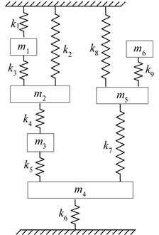
For the verification of the method a six degree of freedom spring-mass system given in Fig. 1 was considered [9-11]. The value of all the masses is 1 kg and the springs’ coefficients are 1 N/m. The natural frequencies of the system are given in Table 1. Receptances of the system were calculated in the frequency band 0-0.35 Hz with a 10^-4 interval. A Matlab code was implemented to apply the proposed method. Eq. (10) was easily created in a single line using a loop. For the solution of nonlinear equations, the fsolve function was used and the initial values were set to zero for all examples. The simulations for different cases were given below.

Fig. 1A six degree of freedoms spring-mass system for numerical simulation

4.3. Case 3. Shifting six natural frequencies

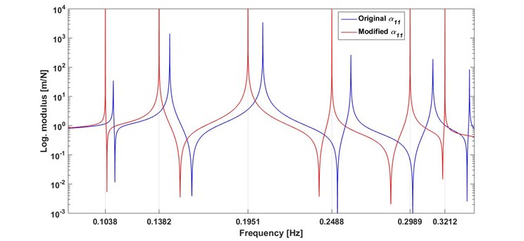
As a last example, all of the six modes are considered to shift to the desired values. For this, all of the masses of the original system are modified with a ratio of 10 %, namely the new values of the masses are 1.1 kg. In this case, the target natural frequencies are determined as {0.1038 0.1382 0.1951 0.2488 0.2989 0.3212}. Then it is desired that the system has these new natural frequencies after six mass modifications. The necessary masses are estimated with a small difference as seen in Table 4. For this case, the receptances of the original and modified systems are also plotted in Fig. 2. As can be seen in the figure that the desired natural frequencies are exactly achieved after modifications.

Table 4Estimated mass modifications for shifting all of the six natural frequencies in the cases of noise-free and noisy receptances

Modification cords.	Estimated mass modifications (kg)
	Noise-free	5 % noise	10 % noise
1	0.09929	0.09779	0.08749
2	0.09944	0.07953	0.14899
3	0.10261	0.11513	0.05638
4	0.09926	0.07231	0.19301
5	0.10067	0.12827	0.00522
6	0.09973	0.09531	0.11755

Fig. 2The receptances of the original and modified systems

In order to verify the efficiency of the proposed method in the case where the receptances are contaminated with noise, as seen in real word applications, the additive white noise with ratios of 5 % and 10 % was added to the receptances of the original system. For these cases, the estimated mass modifications are also given in Table 4 and the receptances are plotted in Fig. 3. For the case of 5 % noise, the results are satisfactory. For the case of 10 % noise, although some masses, especially fourth and fifth masses, are estimated with a large difference, the desired natural frequencies are achieved. However, some spurious picks appear nearby the modes.

5. Experimental study

In this section the efficiency of the proposed method is verified by an experimental study. The test structure is a steel beam which is suspended by a nylon thread as shown in Fig. 4, the dimensions and the mass of the beam are 850×25×12 mm and 2 kg, respectively. In this application, shifting of three natural frequencies case was considered. Three modification locations were chosen and labelled as 1, 2 and 3 on the test beam. The proposed method needs the point FRFs and transfer FRFs related to the modification locations of the beam. In a hammer test, to measure more than one point FRF, it is necessary to move the accelerometer to the measurement points when single accelerometer is used. Moving accelerometer during the measurement of a set of FRFs can yield unexpected results, due to the mass effect of the accelerometer. In order to avoid from this problem, three accelerometers (each one is 5 g in mass) were used to measure FRFs in this study. In this case, even though the mass of the accelerometers affects the system, their effects will be the same on all of the measured FRFs. In this way, the mass effects of the accelerometer on the FRFs are neutralized because they are not moved on the beam to measure point FRFs, and consequently, the effect of the accelerometer on the performance of the method can be minimized. On the other hand, as seen in the numerical simulation, no solution was found, or physically unfeasible solutions were found for some modification locations and for some target natural frequencies. In order to not coincidence with such a case in this experimental study, using the real frequency values would be convenient. Therefore, a simulated test strategy is proposed for the experimental study, similar to the case 2 in the numerical simulations: The beam was first modified by three known dummy masses. Then, the natural frequencies of the modified beam were determined and named as target natural frequencies. The desired natural frequencies were chosen amongst them. It is expected that, the estimated mass modifications by using the proposed method are close to the used dummy masses.

Fig. 3The receptances of the original and modified systems, with a) 5 % noise and b) 10 % noise

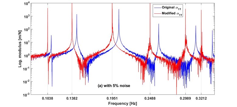
a)

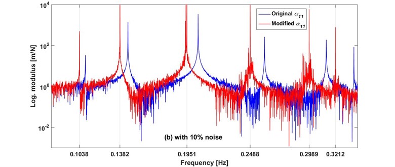
b)

The beam without dummy masses was hit by a modal hammer at locations 1, 2, and 3, respectively and the FRFs were measured in bandwidth 0-1.28 kHz with 0.4 Hz interval. Thus the 3×3 symmetric FRFs matrix was acquired. It should be noted that, in the experiment although the accelerances were measured they were transformed to the receptance to apply the proposed method and they were showed by ${\alpha }_{pq}$ where $p$ and $q$ represent the response and excitation points, respectively. Three of the receptances, which constitute the first row of the measured FRF matrix, are plotted in Fig. 5. Then, for a realistic simulation three dummy masses of 16, 32 and 20 g were located at locations 1, 2 and 3, respectively, as seen in Fig. 4. A FRF was measured to determine the natural frequencies of the modified beam. One of the FRFs of the beam with and without dummy masses is compared in Fig. 6. The natural frequencies of the modified beam tend to decrease as expected. The beam without dummy masses is referred to as the original beam and the beam with dummy masses is referred to as the target beam. The natural frequencies of the original and the target beams are also given in Table 5.

Fig. 4Photography of the test beam, showing the measurement and modification locations

Fig. 5The measured three FRFs of the original beam

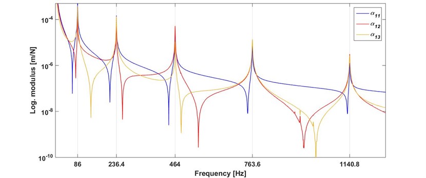
For all of the possible different ten cases, the estimated mass modifications and the determined natural frequencies of the modified beam are tabulated in Table 6. Note that, although the obtained mass modifications are complex the imaginary part was ignored because it is physically unimportant. The first line of the table belongs to the beam modified by known dummy masses, namely the target beam. Although the different mass modifications are found, the target natural frequencies are exactly achieved for each case. However, all of the five natural frequencies are exactly match with those of the target beam for cases 7-9. This is a result of inverse modification problems. For case 7, the target receptance which measured with three dummy masses and the receptance of the beam modified with estimated masses are plotted in Fig. 7. As can be seen, the two receptances are fit together with the exception of antiresonance frequencies. This can be explained as follows: the beam was not able to hit exactly at location 3 because of the attached modification mass at this point.

Fig. 6Comparison of the measured FRFs of original and target beams

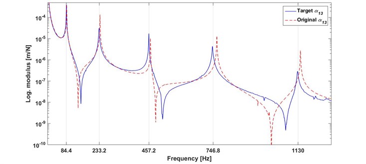
Fig. 7Comparison of a cross receptance of the target and modified beams

It should be noted that, a solution was able to be found for each case of the example above because the chosen target modes belong to a realistic modified beam. But, a solution may not exist or physically unfeasible solutions may be found when the natural frequencies are arbitrarily chosen. For example, to shift natural frequencies to the desired values of {80.0 453.0 1140.0} Hz, the necessary masses are estimated as {–480.3 –112.5 –536.9} g, which are physically inapplicable because the modification masses have a negative sign and have big values compared to the total mass of the beam.

6. Conclusions

This paper focuses on the shifting of a certain number of natural frequencies of a dynamic system to desired values with the concentrated mass modifications. A method based on SM formula is proposed for the calculation of necessary masses. The method uses the receptances of the system relating to the modification coordinates and needs neither the physical mass, the stiffness matrices nor the modal properties. However, an additional degree of freedom is not introduced to the system. The method yields a set of nonlinear equations after the sequential mass modifications at the prespecified coordinates and then the necessary masses are estimated by solving these equations numerically.

The method proposed was first verified by the numerical applications. It is shown that the method is very effective. The excellent results are found for some chosen modification coordinates. However, no solution or physically unfeasible solution is found for some chosen modification coordinates, due to the nature of the inverse modification problem. As known, a mass modification does not affect a mode if it is located at a nodal point of that mode. However, different solutions can be obtained depending on choosing the modification coordinates. The performance of the method was also examined with noisy receptances. Although the method is also effective in the case of noisy FRFs some spurious picks occur nearby natural frequencies, especially when the noise level is high.

The method was also verified by a real beam experiment. Although the proposed method is developed by assuming the system is undamped, the real systems have an amount of damping. In this case, necessary mass modifications are complex values which are physically unimportant, and the imaginary part can be ignored. In spite of that, the results are very satisfactory for the beam that has a small amount of damping. It is concluded that the method can also be used for real structures as long as the noise and damping values are low.