Reconstructing the acoustic far-field using a semi-circular sensor array

1. Introduction

In recent years, the acoustic field reconstruction technique based on near-field measurement has been widely used [1-7]. Near-field measurement can capture evanescent wave signals, so the acoustic reconstruction based on near-field measurement has great advantages in the identification and localization of noise sources. But the acoustic far-field can be reconstructed accurately without evanescent wave. Therefore, there are many disadvantages in the reconstruction of acoustic far-field based on near-field measurement. First, the measuring points for near field measurements are required more. Second, the signal-to-noise ratio of measurement environment is required higher. The acoustic field reconstruction technique based on far field measurements can overcome the above shortcomings. Jiang Zhe proposed using acoustic radiation modes to reconstruct the acoustic field [8]. The acoustic field of two typical sound sources, flat plate and sphere, are reconstructed successfully by this method. Yang Dongsheng has made some applications of acoustic radiation modes to reconstruct the acoustic field of a spherical source [9]. In the arrangement of the far field measuring points, the two Researchers adopt the way of arranging the measuring points evenly on the spherical surface. The advantage of this method of measuring points is to ensure the accuracy of the reconstruction results, but for engineering large-scale structure, this method of measurement is very difficult to implement. In this paper, a method for reconstructing acoustic field by using semi-circular sensor array is proposed, which can reconstruct the acoustic far-field using a simple measuring array. Firstly, the far-field sound pressures are measured using a semi-circular sensor array. Secondly, the far-field of sound sources is reconstructed by theory of acoustic radiation modes. The effectiveness of the proposed method is verified by numerical simulations of rectangular plate acoustic field. The stability of the method is studied when noise is added to the sound pressures at the measuring points.

2. Theory

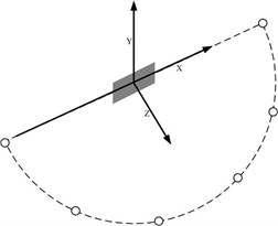
As shown in Fig. 1, a rectangular coordinate system is established by using the geometric center of the sound source as the origin. The semi-circular acoustic pressure sensor array is arranged on the $X$-$Z$ plane. The $n$ far-field pressures are obtained by the $n$ sound pressure sensors on the array. The purpose of this paper is to reconstruct the whole acoustic far-field by the $n$ pressures. Suppose that the measured sound pressure vector is ${\mathbf{p}}_m$, the reconstructed far-field sound pressure vector is ${\mathbf{p}}_f$. The surface of sound source structure is discretized, and suppose that the normal velocity vector on the surface is ${\mathbf{v}}_n$. The sound pressure vector ${\mathbf{p}}_m$ and the velocity vector ${\mathbf{p}}_f$ can be represented by the normal velocity vector on the surface:

where, ${\mathbf{Z}}_1$ is the transfer function matrix between the normal velocity vector of the source surface and the sound pressure vector at the measuring points; ${\mathbf{Z}}_2$ is the transfer function matrix between the normal velocity vector of the source surface and the sound pressure vector at the reconstructed points.

Fig. 1Schematic diagram of the arrangement of sensor array

Based on the theory of acoustic radiation modes, the normal velocity vector of the source surface can be represented by a linear combination of acoustic radiation modal vectors:

In which, $\mathbf{c}$ is the acoustic radiation modal coefficient; $\mathbf{\Phi }$ is the acoustic radiation modal matrix, whose column vector is the acoustic radiation modal vector. The acoustic radiation modal matrix is usually obtained by the eigenvalue decomposition of the radiation resistance matrix. Wu [10] directly computed the acoustic radiation modes which has complex vector form, through the eigenvalue decomposition of radiation impedance matrix. Because the two have the same character, the form of acoustic radiation modes does not affect the effect of acoustic field reconstruction in this paper. Without loss of generality, acoustic radiation modes are obtained by the eigenvalue decomposition of radiation resistance matrix in this paper. Eq. (3) is substituted into Eq. (1) and Eq. (2), the Eq. (1) and the Eq. (2) become:

Define ${\mathbf{\psi }}_1={\mathbf{Z}}_1\mathbf{\Phi }$ and ${\mathbf{\psi }}_2={\mathbf{Z}}_2\mathbf{\Phi }$, ${\mathbf{\psi }}_1$ and ${\mathbf{\psi }}_2$ is the acoustic field distribution modal matrix of measuring points and reconstructing points respectively. Due to the acoustic radiation modes are arranged in order of radiation efficiency, and the radiation efficiency decreases sharply with the increase of order. So only a small amount of acoustic radiation modes in the front can radiate energy into the far field. The far-field sound pressure can be reconstructed with a small amount of acoustic radiation modes, therefore the acoustic radiation modal matrix $\mathbf{\Phi }$ can be truncated. The acoustic field distribution modal matrix of measuring points and reconstructing points would be written as ${\mathbf{\psi }}_1^{\text{'}}$ and ${\mathbf{\psi }}_2^{\text{'}}$ respectively. The Eq. (4) and the Eq. (5) become:

To avoid the underdetermined equation, the number of acoustic radiation modes should be less than or equal to the number of sensors on the array of measurements. Simultaneous Eq. (6) and Eq. (7), the far-field sound pressure vector can be obtained:

where the "+" represents the pseudo inverse of the matrix.

3. Numerical simulation

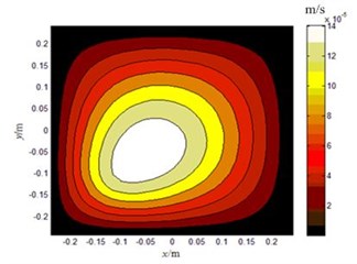
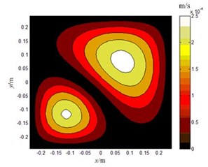
The validity of the proposed method in this paper is certified by a numerical simulation of a plate with infinite baffle. A single point-driven steel plate is selected, the dimensions of the plate are 0.5 m×0.5 m×0.008 m. The baffled plate is modeled in air with 32×32 constant boundary elements, and speed of sound of 340 m/s is assumed for air. When the plate is motivated by the exciting force with a frequency of 100 Hz and 300 Hz respectively, an amplitude of 10 N. The amplitude of the normal velocity on the plate surface is shown in Fig. 2.

Fig. 2The amplitude of normal velocity on the plate surface: a) 100 Hz, b) 300 Hz

a)

b)

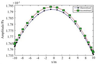
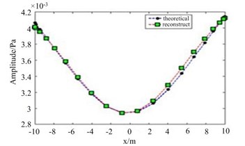
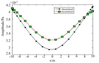
In this simulation, the semi-circular sensor array has a radius of 2 m, and 6 sound pressure sensors are evenly arranged on the semi-circular sensor array. The sound pressures at the measuring points are calculated by Rayleigh integral method. The reconstructed field points are 20 points which distributed evenly on the semi circle of radius 10 m. Using the method introduced in Sec. 2, the sound pressures at the 20 field points are reconstructed. Without loss of generality, the order of the acoustic radiation modes chosen for reconstruction is 6. The reconstructed values of sound pressure are shown in Fig. 3. As seen in Fig. 3, the reconstructed values of sound pressure agree well with the theoretical values whether at 100 Hz or 300 Hz. It is obvious that the far-field pressure reconstruction achieved good results.

To quantify the gap between reconstructed values and theoretical values, define error formula as follows:

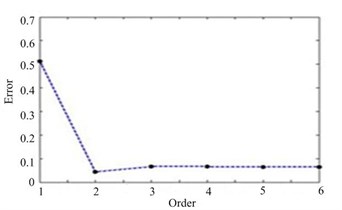
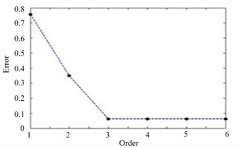
In which, $p_{re}$ and $p_{th}$ is the reconstruction value and the theoretical value respectively. According to Eq. (9), the reconstruction error at 100 Hz is 0.36 %, and the reconstruction error at 300 Hz is 1.62 %. In Fig.4, the variation curve of the reconstruction error with the acoustic radiation modal order is given. As can be seen from Fig. 4, the reconstruction error curve converges quickly. At 100 Hz, the error of the reconstructed sound pressure drops to 1.99 % when the order of the acoustic radiation modes is 2. When the order of the acoustic radiation mode is 3, the error of the reconstructed sound pressure is reduced to 4.72 % at 300 Hz. It shows that only a few acoustic radiation modes contribute to the sound pressure in the far field. The method of acoustic far-field reconstruction using acoustic radiation mode theory has great advantage.

Fig. 3The amplitude of reconstructed pressure: a) 100 Hz, b) 300 Hz

a)

b)

Fig. 4The error curve of reconstructed pressure: a) 100 Hz, b) 300 Hz

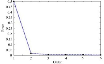
a)

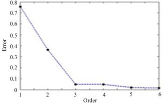
b)

Fig. 5The amplitude of reconstructed pressure in SNR = 15 dB: a) 100 Hz, b) 300 Hz

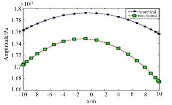
a)

b)

Fig. 6The error curve of reconstructed pressure in SNR = 15 dB: a) 100 Hz, b) 300 Hz

a)

b)

In order to study the stability of the method, a white noise with a signal-to-noise ratio of 15 dB is added to the sound pressure at the measuring point. The reconstructed sound pressure and reconstruction error curve after adding white noise are shown in Fig. 5 and Fig. 6. As can be seen from Fig. 5 and Fig. 6, the addition of white noise in the measurement of sound pressure has a definite effect on the reconstructed results of sound pressure. However, the reconstruction error caused by white noise is small. The reconstruction error at 100 Hz is 6.48 %, and the reconstruction error at 300 Hz is 6.39 %. The reconstruction results are still very accurate. The method is proved to be of good stability.

4. Conclusions

This paper proposes an acoustic far-field reconstruction method using a semi-circular sensor array. Firstly, the pressures in the acoustic far-field are measured by a semi-circular sensor array; then, the acoustic far-field is reconstructed based on the theory of acoustic radiation modes. The numerical simulation of acoustic far-field reconstruction of a rectangular plate is carried out. The result shows that the method can reconstruct the acoustic far-field of the rectangular plate using small number of sensors distributed on a semi-circular array. The numerical simulation results under noise condition show that this method has good stability. This method achieved satisfactory far-field reconstruction accuracy by a simple measuring array. It is especially suitable for the prediction of radiation acoustic field of large structures, and has a good prospect of engineering application.