Multivariant linear regression model based response prediction in situation of unknown uncorrelated multiple sources load

Zhan, Wei; Wang, Cheng

doi:10.21595/vp.2017.19115

Vibroengineering Procedia

Browse Procedia

Published: 21 October 2017

Check for updates

Multivariant linear regression model based response prediction in situation of unknown uncorrelated multiple sources load

Wei Zhan¹

Cheng Wang²

^{1, 2}College of Computer Science and Technology, HuaQiao University, Xiamen, China

Corresponding Author:

Cheng Wang

Cite the article Download PDF

Downloads 1390

CrossRef Citations 2

Abstract

In order to predict response in the situation of unknown uncorrelated multiple sources load, a new response prediction method in frequency domain is proposed. The algorithm needs no transfer function and straightforwardly looking for the inner link between the known responses and the unknown responses. In the multivariant linear regression model, the vibration data of known measuring points are used as input and the vibration data of the unknown measuring points are used as output. And the parameters of multivariant linear regression model are solved by historical training data and the least squares generalized inverse. Experiment verification results of acoustic and vibration sources on cylindrical shell showed that the proposed approach could predict vibration response effectively and satisfy industrial requirements.

1. Introduction

Too large structural vibration response is one of the main reasons for mechanical damage. In frequency domain, there are two common methods to predict response: one is finite element method and another is transfer function based method. And the usage of transfer function and load to predict response is widely used [1, 2]. Wu Z. [3] et al. put up a vibration prediction based on soil frequency response function in frequency domain. Now combining experimental method and finite element method is very popular, Somashekar V. N. [4] et al. put up a new method based on experimentally validate finite element mode to predict printed circuit boards’ vibration response. However, both of these methods can predict response only when the multiple sources load is known. In order to predict the unknown response in the situation of unknown uncorrelated multiple sources load, Mao W. et al. [5] used multiple-input multiple-output SVM model to do load identification. Wang et al [6] used least square generalized inverse to estimate uncorrelated multiple sources load in frequency domain. Based on these reaches, this paper discusses how to use least square generalized inverse to predict the unknown response directly.

2. The theoretical basis of dynamics about loads and responses in frequency domain

2.1. Problem description of response prediction

The question is that now only part of vibration response of measurement points is known. The responses can be classified into the known responses and the unknown responses. Then n response points can be classified into $n_{1}$ known response points and $n_{2}$ unknown response points $(n_{1} + n_{2} = n)$ : the known $n_{1}$ response points $j = 1,2, \dots, n_{1}$ and the unknown $n_{2}$ responses $j = n_{1} + 1, \dots, n_{1} + h, \dots, n_{1} + n_{2}$ , where $h$ from 1 to $n_{2}$ . The vibration response of the $n_{2}$ unknown measurement points should be predicted by vibration response of the $n_{1}$ known measurement points without knowledge of uncorrelated multiple sources load.

2.2. Linear relationship between response and uncorrelated multi-sources

In frequency domain, when the excitations are uncorrelated acted on the linear time invariant system and get multiple responses of the system, the relationship between multiple input and multiple output are linear [9]. Vibration responses of linear time invariant (LTI) system from uncorrelated multiple sources load and multiple measurement points meet the following equation [6]:

1

[\begin{matrix} S_{y_{1} y_{1}} (ω) \\ ⋮ \\ S_{y_{j} y_{j}} (ω) \\ ⋮ \\ S_{y_{n} y_{n}} (ω) \end{matrix}] = [\begin{matrix} {|H_{1,1} (ω)|}^{2} & \dots & {|H_{1, i} (ω)|}^{2} & \dots & {|H_{1, m} (ω)|}^{2} \\ ⋮ & ⋱ & ⋮ & ⋱ & ⋮ \\ {|H_{j, 1} (ω)|}^{2} & \dots & {|H_{j, i} (ω)|}^{2} & \dots & {|H_{j, m} (ω)|}^{2} \\ ⋮ & ⋱ & ⋮ & ⋱ & ⋮ \\ {|H_{n, 1} (ω)|}^{2} & \dots & {|H_{n, i} (ω)|}^{2} & \dots & {|H_{n, m} (ω)|}^{2} \end{matrix}] [\begin{matrix} S_{f_{1} f_{1}} (ω) \\ ⋮ \\ S_{f_{i} f_{i}} (ω) \\ ⋮ \\ S_{f_{m} f_{m}} (ω) \end{matrix}] .

The vibration response of the $n_{1}$ known measurement points must be used to identified the uncorrelated multiple sources load, let:

B (ω) = [\begin{matrix} {|H_{1,1} (ω)|}^{2} & \dots & {|H_{1, i} (ω)|}^{2} & \dots & {|H_{1, m} (ω)|}^{2} \\ ⋮ & ⋱ & ⋮ & ⋱ & ⋮ \\ {|H_{j, 1} (ω)|}^{2} & \dots & {|H_{j, i} (ω)|}^{2} & \dots & {|H_{j, m} (ω)|}^{2} \\ ⋮ & ⋱ & ⋮ & ⋱ & ⋮ \\ {|H_{n_{1}, 1} (ω)|}^{2} & \dots & {|H_{n_{1}, i} (ω)|}^{2} & \dots & {|H_{n_{1}, m} (ω)|}^{2} \end{matrix}],

{\overset{⃑}{S}}_{Y} (ω) = [\begin{matrix} S_{y_{1} y_{1}} (ω) \\ ⋮ \\ S_{y_{j} y_{j}} (ω) \\ ⋮ \\ S_{y_{n_{_{1}}} y_{n_{_{1}}}} (ω) \end{matrix}], {\overset{⃑}{S}}_{F} (w) = [\begin{matrix} S_{f_{1} f_{1}} (ω) \\ ⋮ \\ S_{f_{i} f_{i}} (ω) \\ ⋮ \\ S_{f_{m} f_{m}} (ω) \end{matrix}] .

Liking Eq. (1), it can get the matrix form as:

2

{\vec{S}}_{Y} (ω) = B (ω) {\vec{S}}_{F} (ω) .

2.3. Procedure of known responses based response prediction in situation of unknown uncorrelated multi-sources and with knowledge of transfer functions

Step 1): Obtaining the transfer functions module $B (ω)$ of the linear time invariant system from uncorrelated multiple loads to known measurement points and unknown measurement points. And The obtainment of transfer functions can be classified in two ways [7-8].

Step 2): Using transfer functions module $B (ω)$ from uncorrelated multiple loads to known measurement points and known measurement points ${\overset{⃑}{S}}_{Y} (ω)$ to identify uncorrelated multi-source loads ${\vec{S}}_{F} (ω)$ by least-squares of generalized matrix inverse method, the uncorrelated multi-source loads can be identified through the system’s transfer functions of all uncorrelated multi-source loads to all the known measurement points and the vibration response of the $n_{1}$ known measurement points [9]:

3

{\hat{\vec{S}}}_{F} (ω) = B^{+} (ω) {\overset{⃑}{S}}_{Y} (ω) = {[B^{T} (ω) B (ω)]}^{- 1} B^{T} (ω) {\overset{⃑}{S}}_{Y} (ω),

where $B^{+} (ω) ≜ {[B^{T} (ω) B (ω)]}^{- 1} B^{T} (ω)$ is the least square generalized inverse of $B (ω)$ .

Step 3): Unknown measurement points Vibration response prediction based on transfer functions from uncorrelated multi-source loads to unknown measurement points and the identified uncorrelated multi-source loads ${\hat{\vec{S}}}_{F} (ω)$ .

After identifying the uncorrelated multi-source loads, the vibration response of the unknown measurement points can be predicted by Eq. (4):

4

[\begin{matrix} {\hat{S}}_{y_{n_{1} + 1} y_{n_{1} + 1}}^{u n k n o w n} (ω) \\ ⋮ \\ {\hat{S}}_{y_{_{n_{1 + h}}} y_{n_{1 + h}}}^{u n k n o w n} (ω) \\ ⋮ \\ {\hat{S}}_{y_{n_{1} + n_{2}} y_{_{n_{1} + n_{2}}}}^{u n k n o w n} (ω) \end{matrix}] = [\begin{matrix} {|H_{n_{1} + 1,1} (ω)|}^{2} & \dots & {|H_{n_{1} + 1, i} (ω)|}^{2} & \dots & {|H_{n_{1} + 1, m} (ω)|}^{2} \\ ⋮ & ⋱ & ⋮ & ⋱ & ⋮ \\ {|H_{n_{1} + h, 1} (ω)|}^{2} & \dots & {|H_{n_{1} + h, i} (ω)|}^{2} & \dots & {|H_{n_{1} + h, m} (ω)|}^{2} \\ ⋮ & ⋱ & ⋮ & ⋱ & ⋮ \\ {|H_{n_{1} + n_{2}, 1} (ω)|}^{2} & \dots & {|H_{n_{1} + n_{2}, i} (ω)|}^{2} & \dots & {|H_{n_{1} + n_{2}, m} (ω)|}^{2} \end{matrix}] [\begin{matrix} {\hat{S}}_{f_{1} f_{1}}^{} (ω) \\ ⋮ \\ {\hat{S}}_{f_{i} f_{i}}^{} (ω) \\ ⋮ \\ {\hat{S}}_{f_{m} f_{m}}^{} (ω) \end{matrix}] .

3. Procedure of known responses based unknown response prediction

3.1. The formula derivation of the linear relationship between known response and unknown response

After plugging the identified uncorrelated multiple sources load of Eq. (3) into Eq. (4), the vibration response of the unknown measurement points can be predicted by the known response:

5

[\begin{matrix} {\hat{S}}_{y_{n_{1} + 1} y_{n_{1} + 1}}^{} (ω) \\ ⋮ \\ {\hat{S}}_{y_{_{n_{1 + h}}} y_{n_{1 + h}}}^{} (ω) \\ ⋮ \\ {\hat{S}}_{y_{n_{1} + n_{2}} y_{_{n_{1} + n_{2}}}}^{} (ω) \end{matrix}] = [\begin{matrix} {|H_{n_{1} + 1,1} (ω)|}^{2} & \dots & {|H_{n_{1} + 1, i} (ω)|}^{2} & \dots & {|H_{n_{1} + 1, m} (ω)|}^{2} \\ ⋮ & ⋱ & ⋮ & ⋱ & ⋮ \\ {|H_{n_{1} + h, 1} (ω)|}^{2} & \dots & {|H_{n_{1} + h, i} (ω)|}^{2} & \dots & {|H_{n_{1} + h, m} (ω)|}^{2} \\ ⋮ & ⋱ & ⋮ & ⋱ & ⋮ \\ {|H_{n_{1} + n_{2}, 1} (ω)|}^{2} & \dots & {|H_{n_{1} + n_{2}, i} (ω)|}^{2} & \dots & {|H_{n_{1} + n_{2}, m} (ω)|}^{2} \end{matrix}] [\begin{matrix} {\hat{S}}_{f_{1} f_{1}}^{} (ω) \\ ⋮ \\ {\hat{S}}_{f_{i} f_{i}}^{} (ω) \\ ⋮ \\ {\hat{S}}_{f_{m} f_{m}}^{} (ω) \end{matrix}]

= [\begin{matrix} {|H_{n_{1} + 1,1} (ω)|}^{2} & \dots & {|H_{n_{1} + 1, i} (ω)|}^{2} & \dots & {|H_{n_{1} + 1, m} (ω)|}^{2} \\ ⋮ & ⋱ & ⋮ & ⋱ & ⋮ \\ {|H_{n_{1} + h, 1} (ω)|}^{2} & \dots & {|H_{n_{1} + h, i} (ω)|}^{2} & \dots & {|H_{n_{1} + h, m} (ω)|}^{2} \\ ⋮ & ⋱ & ⋮ & ⋱ & ⋮ \\ {|H_{n_{1} + n_{2}, 1} (ω)|}^{2} & \dots & {|H_{n_{1} + n_{2}, i} (ω)|}^{2} & \dots & {|H_{n_{1} + n_{2}, m} (ω)|}^{2} \end{matrix}]

∙ {[\begin{matrix} {|H_{1,1} (ω)|}^{2} & \dots & {|H_{1, i} (ω)|}^{2} & \dots & {|H_{1, m} (ω)|}^{2} \\ ⋮ & ⋱ & ⋮ & ⋱ & ⋮ \\ {|H_{j, 1} (ω)|}^{2} & \dots & {|H_{j, i} (ω)|}^{2} & \dots & {|H_{j, m} (ω)|}^{2} \\ ⋮ & ⋱ & ⋮ & ⋱ & ⋮ \\ {|H_{n_{1}, 1} (ω)|}^{2} & \dots & {|H_{n_{1}, i} (ω)|}^{2} & \dots & {|H_{n_{1}, m} (ω)|}^{2} \end{matrix}]}^{+} [\begin{matrix} S_{y_{1} y_{1}} (ω) \\ ⋮ \\ S_{y_{j} y_{j}} (ω) \\ ⋮ \\ S_{y_{n_{_{1}}} y_{n_{_{1}}}} (ω) \end{matrix}] .

Let:

D (ω) ≜ [\begin{matrix} D_{n_{1} + 1,1} (ω) & \dots & D_{n_{1} + 1, j} (ω) & \dots & D_{n_{1} + 1, n_{1}} (ω) \\ ⋮ & ⋱ & ⋮ & ⋱ & ⋮ \\ D_{n_{1} + h, 1} (ω) & \dots & D_{n_{1} + h, j} (ω) & \dots & D_{n_{1} + h, n_{1}} (ω) \\ ⋮ & ⋱ & ⋮ & ⋱ & ⋮ \\ D_{n_{1} + n_{2}, 1} (ω) & \dots & D_{n_{1} + n_{2}, j} (ω) & \dots & D_{n_{1} + n_{2}, n_{1}} (ω) \end{matrix}]

≜ [\begin{matrix} | H_{n_{1} + 1,1} (ω) |^{2} & \dots & | H_{n_{1} + 1, i} (ω) |^{2} & \dots & | H_{n_{1} + 1, m} (ω) |^{2} \\ ⋮ & ⋱ & ⋮ & ⋱ & ⋮ \\ | H_{n_{1} + h, 1} (ω) |^{2} & \dots & | H_{n_{1} + h, i} (ω) |^{2} & \dots & | H_{n_{1} + 1, m} (ω) |^{2} \\ ⋮ & ⋱ & ⋮ & ⋱ & ⋮ \\ | H_{n_{1} + n_{2}, 1} (ω) |^{2} & \dots & | H_{n_{1} + n_{2}, i} (ω) |^{2} & \dots & | H_{n_{1} + n_{2}, m} (w) |^{2} \end{matrix}]

∙ {[\begin{matrix} | H_{1,1} (ω) |^{2} & \dots & | H_{1, i} (ω) |^{2} & \dots & | H_{1, m} (ω) |^{2} \\ ⋮ & ⋱ & ⋮ & ⋱ & ⋮ \\ | H_{j, 1} (ω) |^{2} & \dots & | H_{j, i} (ω) |^{2} & \dots & | H_{j, m} (ω) |^{2} \\ ⋮ & ⋱ & ⋮ & ⋱ & ⋮ \\ | H_{n_{1}, 1} (ω) |^{2} & \dots & | H_{n_{1}, i} (ω) |^{2} & \dots & | H_{n_{1}, m} (ω) |^{2} \end{matrix}]}^{+} \in R^{n_{2} \times n_{1}} .

So, Eq. (6) can be obtained from Eq. (5):

6

[\begin{matrix} S_{y_{n_{1} + 1} y_{n_{1} + 1}} (ω) \\ ⋮ \\ S_{y_{n_{1} + h} y_{_{n_{1} + h}}} (ω) \\ ⋮ \\ S_{y_{n_{1} + n_{2}} y_{_{n_{1} + n_{2}}}} (ω) \end{matrix}] = [\begin{matrix} D_{n_{1} + 1,1} (ω) & \dots & D_{1, j} (ω) & \dots & D_{1, n_{1}} (ω) \\ ⋮ & ⋱ & ⋮ & ⋱ & ⋮ \\ D_{n_{1} + h, 1} (ω) & \dots & D_{n_{1} + h, j} (ω) & \dots & D_{n_{1} + h, n_{1}} (ω) \\ ⋮ & ⋱ & ⋮ & ⋱ & ⋮ \\ D_{n_{1} + n_{2}, 1} (ω) & \dots & D_{n_{1} + n_{2}, j} (ω) & \dots & D_{n_{1} + n_{2}, n_{1}} (ω) \end{matrix}] [\begin{matrix} S_{y_{1} y_{1}} (ω) \\ ⋮ \\ S_{y_{j} y_{j}} (ω) \\ ⋮ \\ S_{y_{n_{1}} y_{n_{1}}} (ω) \end{matrix}] .

Until now, the linear relationship between the known responses and the unknown response on the LTI system in frequency domain is clear. Eq. (7) can be obtained from Eq. (6). For the row $h$ of Eq. (6), $h = 1,2, \dots, n_{2}$ :

7

S_{y_{n_{1} + h} y_{_{n_{1} + h}}} (ω) = D_{n_{1} + h, 1} (ω) S_{y_{1} y_{1}} (ω) + \dots + D_{n_{1} + h, j} (ω) S_{y_{j} y_{j}} (ω)

+ \dots + D_{n_{1} + h, n_{1}} (ω) S_{y_{n_{1}} y_{n_{1}}} (ω) .

Through $p$ times independent experiment, $q = 1,2, \dots, p$ , the formula of the matrix equation can be obtained:

8

[\begin{matrix} S_{y_{n_{1} + h} y_{_{n_{1} + h}}}^{1} (ω) \\ ⋮ \\ S_{_{y_{n_{1} + h} y_{_{n_{1} + h}}}}^{q} (ω) \\ ⋮ \\ S_{y_{n_{1} + h} y_{_{n_{1} + h}}}^{p} (ω) \end{matrix}] = [\begin{matrix} S_{y_{1} y_{1}}^{1} (ω) & \dots & S_{y_{j} y_{j}}^{1} (ω) & \dots & S_{y_{n_{1}} y_{n_{1}}}^{1} (ω) \\ ⋮ & ⋱ & ⋮ & ⋱ & ⋮ \\ S_{y_{1} y_{1}}^{q} (ω) & \dots & S_{y_{j} y_{j}}^{q} (ω) & \dots & S_{y_{n_{1}} y_{n_{1}}}^{q} (ω) \\ ⋮ & ⋱ & ⋮ & ⋱ & ⋮ \\ S_{y_{1} y_{1}}^{p} (ω) & \dots & S_{y_{j} y_{j}}^{p} (ω) & \dots & S_{y_{n_{1}} y_{n_{1}}}^{p} (ω) \end{matrix}] [\begin{matrix} D_{n_{1} + h, 1} (ω) \\ ⋮ \\ D_{n_{1} + h, j} (ω) \\ ⋮ \\ D_{n_{1} + h, n_{1}} (ω) \end{matrix}] .

The coefficient of ${[{\hat{D}}_{n_{1} + h, 1} (ω), \dots, {\hat{D}}_{n_{1} + h, i} (ω), \dots, {\hat{D}}_{n_{1} + h, n_{1}} (ω)]}^{T}$ can be obtained only when $p \geq n_{1}$ , and its least square solution is:

9

[\begin{matrix} {\hat{D}}_{n_{1} + h, 1} (ω) \\ ⋮ \\ {\hat{D}}_{n_{1} + h, j} (ω) \\ ⋮ \\ {\hat{D}}_{n_{1} + h, n_{1}} (ω) \end{matrix}] = {[\begin{matrix} S_{y_{1} y_{1}}^{1} (ω) & \dots & S_{y_{j} y_{j}}^{1} (ω) & \dots & S_{y_{n_{1}} y_{n_{1}}}^{1} (ω) \\ ⋮ & ⋱ & ⋮ & ⋱ & ⋮ \\ S_{y_{1} y_{1}}^{q} (ω) & \dots & S_{y_{j} y_{j}}^{q} (ω) & \dots & S_{y_{n_{1}} y_{n_{1}}}^{q} (ω) \\ ⋮ & ⋱ & ⋮ & ⋱ & ⋮ \\ S_{y_{1} y_{1}}^{p} (ω) & \dots & S_{y_{j} y_{j}}^{p} (ω) & \dots & S_{y_{n_{1}} y_{n_{1}}}^{p} (ω) \end{matrix}]}^{+} [\begin{matrix} S_{y_{n_{1} + h} y_{_{n_{1} + h}}}^{1} (ω) \\ ⋮ \\ S_{_{y_{n_{1} + h} y_{_{n_{1} + h}}}}^{q} (ω) \\ ⋮ \\ S_{y_{n_{1} + h} y_{_{n_{1} + h}}}^{p} (ω) \end{matrix}] .

Likely, all rows of $D (ω)$ can be solved in the same way, $h = 1,2, \dots, n_{2}$ . Then, the vibration response of the unknown measurement points can be predicted by the vibration of the known measurement points through Eq. (10):

10

[\begin{matrix} S_{y_{n_{1} + 1} y_{n_{1} + 1}}^{u n k n o w n} (ω) \\ ⋮ \\ S_{y_{n_{1} + h} y_{_{n_{1} + h}}}^{u n k n o w n} (ω) \\ ⋮ \\ S_{y_{n_{1} + n_{2}} y_{_{n_{1} + n_{2}}}}^{u n k n o w n} (ω) \end{matrix}] = [\begin{matrix} D_{n_{1} + 1,1} (ω) & \dots & D_{1, j} (ω) & \dots & D_{1, n_{1}} (ω) \\ ⋮ & ⋱ & ⋮ & ⋱ & ⋮ \\ D_{n_{1} + h, 1} (ω) & \dots & D_{n_{1} + h, j} (ω) & \dots & D_{n_{1} + h, n_{1}} (ω) \\ ⋮ & ⋱ & ⋮ & ⋱ & ⋮ \\ D_{n_{1} + n_{2}, 1} (ω) & \dots & D_{n_{1} + n_{2}, j} (ω) & \dots & D_{n_{1} + n_{2}, n_{1}} (ω) \end{matrix}] [\begin{matrix} S_{y_{1} y_{1}}^{k n o w n} (ω) \\ ⋮ \\ S_{y_{j} y_{j}}^{k n o w n} (ω) \\ ⋮ \\ S_{y_{n_{1}} y_{n_{1}}}^{k n o w n} (ω) \end{matrix}] .

Since the linear relationship between known responses and unknown responses is clear, multivariant linear regression can be used to construct the modal and least squares method can be applied to solve this modal without knowledge of transfer functions.

3.2. Procedure of known responses based to predict unknown responses directly

Step 1): Training modal construction. In training modal, the responses must be classified in to two parts. One is known responses and the other is unknown responses.

Step 2): The solution of the linear relationship matrix $D (ω)$ between the known responses and the unknown response. Since we get that the relationship between the known responses and the unknown responses is linear, the least square method is used to get the linear relation matrix $D (ω)$ through Eq. (10).

Step 3): After get the inner link matrix $D (ω)$ , the unknown responses can be predicted through the known responses by using Eq. (11). So as though the uncorrelated loads and transfer functions are unknown, but in this method it doesn’t need any information of the multi-source loads.

4. Experimental verification

4.1. Acoustic and vibration experiment devices

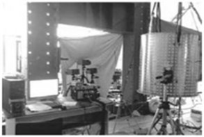
The experiment device is in Figs. 1-3. In the internal of cylindrical shell, there is an acoustic reverberation acoustic excitation as shown in Fig. 1. And in the external, there is a vibration excitation of vibration excitation of vibration table which included a sensor recording the vibration excitation, the external acoustic excitation and the vibration response of surface and inner device as shown in Fig. 2. The arrangement of measuring points as shown in Fig. 3. In the experiments, it could be thought that there are only two independent excitation sources and 18 sensors to measure the vibration responses data in which some data is known and the rest is unknown, using the known vibration data to predict the unknown responses data is what should be done. In the experiment, there were 15 acoustic and vibration union excitation magnitude gradually increased. In all the 15 pair experiment, 14 pair is chosen for training and leave one pair for testing. So that means the independent experiment time p equals to 14 and in order to satisfy the constrain of the applicable scope, we made n equal to 9 (the 9 points are on the upper part of the cylinder), and when predict multiple response at a time, we made the number of known points to 7 and the number of unknown point to 2.

Fig. 1Acoustic excitation

Fig. 2Cylindrical shell measuring points

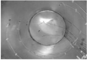
Fig. 3Structure surface

4.2. Experimental evaluation index

To validate the correctness and precision of this method, the predicted response must compare with the real response and 3 dB relative error is widely used in engineering practice. Given prediction response ${\hat{y}}_{k}$ and the real response $y_{k}$ , to satisfy the 3 dB relative error, the condition as follows:

11

10 l o g_{10} |\frac{{\hat{y}}_{k}}{y_{k}}| \leq 3 and 10 l o g_{10} {|\frac{y_{k}}{{\hat{y}}_{k}}|}_{i = 1}^{N} \leq 3 .

4.3. Experiment results

To validate the correctness and precision of the proposed method, the chosen unknown responses compare with the real responses. Because there are total 15 pair experiment and 9 response points, for predicting one point, there are 15×9 = 135 conditions to compare the real responses to the predicted response. In order to make it short, we only express one pair’s result for comparing. Table 1 shows when one point response is unknown, the result of the predict response comparing with the real response. t stands for the unknown point’s number.

When more than one response points predicted, the conditions will be much more than just one unknown point response. For convenience, just 2 point at random in a pair to compare the predict response with the real response are chose. Table 2 shows the result of the comparison, each $t_{1}$ and $t_{2}$ combined to a group. To make it more clear, Fig. 4 shows the energy dB of the predict response and the real response.

Table 1The energy of error over 3 dB of predict response and real response %

$t$	1	2	3	4	5	6	7	8	9
> 3 dB	1.00	4.75	1.50	1.00	1.06	1.25	1.44	0.44	1.31
< –3 dB	4.62	5.25	2.50	2.75	2.19	3.44	2.50	2.25	2.12
Total	5.62	9.99	4.00	3.75	3.25	4.68	3.94	2.69	3.44

Table 2The energy of error over 3 dB of predict response and real response %

	$t_{1}$	$t_{2}$	$t_{1}$	$t_{2}$	$t_{1}$	$t_{2}$
	1	5	2	6	8	9
> 3 dB	0.94	1.00	4.68	1.37	0.81	1.31
< –3 dB	3.25	2.00	4.25	2.50	2.50	1.94
Total	4.18	3.00	8.93	3.87	3.31	3.25

Fig. 4The energy dB of the predict response compare with the real response

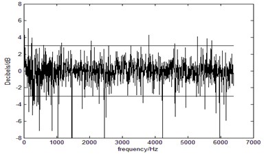
a) $t_{1}$ energy dB comparison

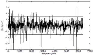
b) $t_{2}$ energy dB comparison

4.4. Experimental results analysis

As it shows above, the proposed method applicable in situation of unknown loads and unknown transfer functions and the accuracy can satisfy the industry standard. Experimental results show that the prediction response is very close to the real response. And the error lies in:

1) In the real experiment there exist noises and other aspects of data error.

2) The ill-condition of matrix inverse problem is another reason of the error between prediction response and the real response [7].

3) The weak nonlinearity of the system also causes the difference between the predicted response and the real response.

5. Conclusions

Least square generalized inverse based algorithm is introduced to response prediction algorithm in frequency domain when uncorrelated multiple sources load are unknown. And with no transfer functions data this method can predict the response effectively. Response prediction experiment verification results of acoustic and vibration sources on cylindrical shell showed effective and higher accuracy of the proposed approach. But this method can only solve the response prediction of linear system, how to predict nonlinear system’s response is future research direction. If the load sources are correlated to each other in frequency domain, the phase of loads and responses will be very important. How to characterize the phase of load and correlated load sources which are also further research direction based multi-source dynamic random response prediction algorithm in frequency domain.

References

Paik I., Roesset J. M. Use of quadratic transfer functions to predict response of tension leg platforms. Journal of Engineering Mechanics, Vol. 122, Issue 9, 1996, p. 882-889.

Publisher
Albert C. G., Veronesi G., Nijman E., et al. Prediction of the vibro-acoustic response of a structure-liner-fluid system based on a patch transfer function approach and direct experimental subsystem characterization. Applied Acoustics, Vol. 112, 2016, p. 14-24.

Publisher
Wu Z. Z., Liu W. N., Ma L. X., et al. Prediction method for metro environmental vibrations based on measured frequency response functions. Engineering Mechanics, 2015.

Search CrossRef
Somashekar V. N., Harikrishnan S., Ahmed P. S. M. A., et al. Vibration response prediction of the printed circuit boards using experimentally validated finite element model. Procedia Engineering, Vol. 144, 2016, p. 576-583.

Publisher
Mao W., Tian M., Yan G. Research of load identification based on multiple-input multiple-output SVM model selection. Journal of Mechanical Engineering Science, Vol. 226, Issue 5, 2012, p. 1395-1409.

Publisher
Wang Cheng, Wu Yongxiang, Jiao Jixiang, Huang Xianglong, Gou Jin, Yan Guirong Load identification of acoustic and vibration multi-source following linear regression and least-squares of generalized matrix inverse method in frequency domain. Sensors and Transducers, Vol. 168, Issue 4, 2014, p. 268-275.

Search CrossRef
Wang Jianying, Wang Cheng, Zhong Bineng, Wang Tian Uncorrelated multi-sources load identification in frequency domain based on improved tikhonov regularization method. International Journal of Applied Electromagnetics and Mechanics, Vol. 52, 2016, p. 983-990.

Publisher
Nishimoto H., Akagi M., Kitamura T., et al. Estimation of transfer function of vocal tract extracted from MRI data by FEM. IEICE Technical Report Speech, Vol. 103, 2004, p. 31-36.

Search CrossRef

Cited by

MIMO LS-SVR-Based Multi-Point Vibration Response Prediction in the Frequency Domain

(2020)

Elastic-net regularization based multi-point vibration response prediction in situation of unknown uncorrelated multiple sources load

(2020)

About this article

Received

14 September 2017

Accepted

24 September 2017

Published

21 October 2017

SUBJECTS

Acoustics, noise control and engineering applications

DOI

https://doi.org/10.21595/vp.2017.19115

Keywords

response prediction in frequency domain

unknown uncorrelated multiple sources

multivariant linear regression model

least squares generalized inverse

Acknowledgements

This research was supported by National Natural Science Foundation of China (Grant No. 51305142, 51305143), the General Financial Grant from the China Postdoctoral Science Foundation (Grant No. 2014M552429).

This is an open access article distributed under the Creative Commons Attribution License, which permits unrestricted use, distribution, and reproduction in any medium, provided the original work is properly cited.

Previous article in issue Previous Next article in issue Next

Research article

2022 06 13

Prediction of structural dynamic response based on transfer function

Lejun Wei, Yinfeng Dong, Hui Tian

Research article

2019 11 15

Chaotic time series prediction using wavelet transform and multi-model hybrid method

Tian Feng, Shuying Yang, Feng Han

Research article

2018 02 15

Wake and structure model for simulation of cross-flow/in-line vortex induced vibration of marine risers

Younes Komachi, Said Mazaheri, Mohammad R. Tabeshpour

Research article

2016 11 15

Dynamic response prediction of non-obstructive particle damping using principles of gas-solid flows

Xiaofei Lei, Chengjun Wu

W. Zhan and C. Wang, “Multivariant linear regression model based response prediction in situation of unknown uncorrelated multiple sources load,” Vibroengineering PROCEDIA, Vol. 14, pp. 271–277, Oct. 2017, https://doi.org/10.21595/vp.2017.19115

Copy Extrica

Copied to clipboard!

TY  - JOUR
DO  - 10.21595/vp.2017.19115
UR  - https://doi.org/10.21595/vp.2017.19115
TI  - Multivariant linear regression model based response prediction in situation of unknown uncorrelated multiple sources load
T2  - Vibroengineering PROCEDIA
AU  - Wang, Cheng
AU  - Zhan, Wei
PY  - 2017
DA  - 2017/10/21
PB  - JVE International Ltd.
SP  - 271-277
VL  - 14
SN  - 2345-0533
ER  - 

Copy Ris

Copied to clipboard!

@article{Wang_2017,
	doi = {10.21595/vp.2017.19115},
	url = {https://doi.org/10.21595/vp.2017.19115},
	year = 2017,
	month = {oct},
	publisher = {{JVE} International Ltd.},
	volume = {14},
	pages = {271--277},
	author = {Cheng Wang and Wei Zhan},
	title = {Multivariant linear regression model based response prediction in situation of unknown uncorrelated multiple sources load},
	journal = {Vibroengineering {PROCEDIA}}
}

Copy Bibtex

Copied to clipboard!

[1]C. Wang and W. Zhan, “Multivariant linear regression model based response prediction in situation of unknown uncorrelated multiple sources load,” Vibroengineering PROCEDIA, vol. 14, pp. 271–277, Oct. 2017, doi: 10.21595/vp.2017.19115.

Copy IEEE

Copied to clipboard!

Wang, Cheng, and Wei Zhan. “Multivariant Linear Regression Model Based Response Prediction in Situation of Unknown Uncorrelated Multiple Sources Load.” Vibroengineering PROCEDIA 14 (October 21, 2017): 271–77. https://doi.org/10.21595/vp.2017.19115.

Copy Chicago

Copied to clipboard!

Multivariant linear regression model based response prediction in situation of unknown uncorrelated multiple sources load

Abstract

1. Introduction

2. The theoretical basis of dynamics about loads and responses in frequency domain

2.1. Problem description of response prediction

2.2. Linear relationship between response and uncorrelated multi-sources

2.3. Procedure of known responses based response prediction in situation of unknown uncorrelated multi-sources and with knowledge of transfer functions

3. Procedure of known responses based unknown response prediction

3.1. The formula derivation of the linear relationship between known response and unknown response

3.2. Procedure of known responses based to predict unknown responses directly

4. Experimental verification

4.1. Acoustic and vibration experiment devices

4.2. Experimental evaluation index

4.3. Experiment results

4.4. Experimental results analysis

5. Conclusions

References

Cited by

About this article

Related Articles