Modeling and simulations on automated vehicles to alleviate traffic congestion

1. Introduction

The problem studied in this paper is from COMAP’s Mathematical Contest in Modeling 2017. It’s about how self-driving cars or automated vehicles impact traffic in certain areas of America. “Automated vehicles” are vehicles that drive themselves and have an automated speed choice. They can drive closer together and at more uniform speeds than human driven cars. Automated vehicle technologies have the potential to improve traffic efficiency, stability and safety [1]. It is necessary to research on the behavior of these cars when interacting with existing traffic flows and with each other. The latest experiment at the California PATH showed that vehicles in platoons can maintain a time gap as small as 0.6 s, compared to 1.5 s for conventional regular vehicles, which implies a substantial increase in roadway capacity and mitigation of drastic congestion [2]. Talebpour et al. examined the impacts of reserving one lane of a four-lane highway for automated vehicles on traffic flow dynamics and travel time reliability. It was found that throughput can be improved significantly if the percentage of automated vehicles is greater than 30 % [3].

Nowadays, very limited theoretical research has been conducted to provide a systematic formulation. To fill this gap, this paper provides a general theoretical framework to show how traffic capacity will change with the introduction of automated vehicles. Particularly, this paper focuses on deriving the base macroscopic capacity for mixed traffic. It is important because the base capacity is varying by a number of factors, which presents complexity in understanding the capacity.

This paper is organized as follows. Section 2 presents a macroscopic traffic flow differential equation model based on automated vehicles to reveal the dynamic evolution of traffic flow. Section 3 presents the aggregate objective function ($AOF$), taking actual expected speed ratio, change lane count, backward distance and overtake as four indicators to study the impact of different proportions of automated vehicles on road capacity. Section 4 establishes the cellular automaton model to study the effect of lane changing strategy on traffic flow. In Section 5, we select several locations randomly to test the reliability of the model. Concluding remarks are provided in Section 6.

2. Macroscopic traffic flow differential equation model for automated vehicles

We divide the road into $m$ sections, and define the length of each section is $L_i$. Assuming that driving on these sections are all automated vehicles, $n_i$ indicates the number of automated vehicles in section $i$.

The classical PI control algorithm is as follow [4]:

where ${\alpha }_{f,i}$ is the throttle input opening angle of car $i$, ${\alpha }_0$ is the nominal value corresponding to the throttle opening angle, and ${\delta }_i$, $v_{rel,i}$ are the pitch error and relative speed of car $i$:

Without considering the braking effect [5], the relationship between the acceleration and throttle opening angle is obtained:

where $a$, $b$ are parameters that vary with speed, and $d$ is model uncertainty.

Substituting Eq. (1) into Eq. (4):

Without loss of generality [6], let:

Eq. (6) becomes:

Eq. (7) is written as follow:

According to the hypothesis, all the cars are satisfied with Eq. (8). In order to obtain the corresponding macroscopic characteristics of traffic flow, all vehicles in each section of the road are collected and processed according to Eq. (5). Take the first section as an example:

Expanding the first and second item on the left of Eq. (9):

where $\stackrel{-}{u}\left(x_1,x_2,t\right)$ is the average speed of section $[x1$, $x2]$.

Expanding the first item on the right of Eq. (9):

The relationship between the actual speed and expeted speed of the automated vehicles can be approximated as [7]:

where $v_{i,des}$ is the expected speed of car $i$.

For an automated vehicle, the relationship between the actual speed and expected speed can be approximated as [8]:

where $s$ is the Laplace operator.

Therefore, the first item on the right of Eq. (12) is converted to:

In the steady state, the number of vehicles in the first section is equal to the number of vehicles in the second section. That is $n_1=n_2$. Therefore, Eq. (15) can also be written as:

Carry out the McLaughlin order expansion on $1/(\tau s+1{)}^{n_1-1}$. Since $\tau <$ 1, we ignore the higher order terms of $\tau$ and obtain:

Substituting Eq. (12) into Eq. (13) to obtain:

Let:

Substituting Eq. (18) into Eq. (12) to obtain:

The $u_{f,2}$ is satisfied with:

Then, the second item on the right of Eq. (9) is expanded, obtaining:

where $L_1$ is the length of section one. $\stackrel{-}{\rho }$($x_1$, $x_2$, $t$) is the average traffic volume in section [$x_1$, $x_2$] at time $t$. The third item on the right of Eq. (9) is expanded, obtaining:

Let:

Substituting Eq. (21) and Eq. (22) into Eq. (23) to obtain:

Substituting Eq. (10), (11), (12), (22) and Eq. (24) into Eq. (9) to obtain the macroscopic characteristic of section one:

For one-dimensional traffic flow, traffic volume and traffic density always satisfy the following conservation equation [9]:

where $\rho \left(x,t\right)$ is the instantaneous velocity at time $t$ in the position $x$, and $q\left(x,t\right)$ is the instantaneous flow rate at time $t$ in the position $x$.

We can obtain:

where $\stackrel{-}{q}$($x_1$, $t$) is the flow rate per unit time into section [$x_1$, $x_2$], and $\stackrel{-}{q}$($x_2$, $t$) is the flow rate per unit time out section [$x_1$, $x_2$].

The form of Eq. (28) in general form:

For the $i$ section, traffic volume is not only related to the average speed and average density of the road section, but also related to the $i-1$ section’s macroscopic characteristic:

where ${\alpha }_x$ is the parameter between 0 and 1. It has been generally believed that the average volume of each section is more dependent on its own section. Hence, the result of ${\alpha }_x$ is closer to 1.

Substituting Eq. (30) into Eq. (29) obtains:

For the first and last section of the road, the boundary conditions are satisfied:

Therefore, we obtain the first and last section average density equation:

In summary, the conclusion shows that the macroscopic traffic flow differential equation model of automated vehicles is:

As can be observed from Eq. (37) that the average speed of section $i$ is mainly determined by three parts: the first part is the influence of the average speed of the upstream section; the second part is the low frequency component of the mean velocity in section $i+1$ of the downstream section, indicating the effect of the average speed of the downstream section; the third part is the expected vehicle spacing.

In summary, Eq. (37)-Eq. (42) are macroscopic traffic flow model based on automated vehicles. This model is combined with the basic characteristics of automated vehicles and traffic flow. From the macroscopic point of view, this model describes the dynamic evolution law of the average density and average speed of the flow of automated vehicles. Taking into account the effect of the upper and lower ramp of the traffic density, this would influence and induce the further study of traffic flow using automated vehicles.

3. Traffic flow evaluation model

4. Cellular automaton model

The basic cellular automaton model is a stochastic traffic flow simulation model. The NaSch model of a single lane is defined in a one-dimensional array of length $L$. Each space of the array is called a cell, which is occupied by a vehicle at most.

Each vehicle's speed range is between 0 and $v_{\mathrm{m}\mathrm{a}\mathrm{x}}$, where $v_{\mathrm{m}\mathrm{a}\mathrm{x}}$ is the highest speed. Each update of the system represents the time forward of a unit. Each update includes four steps, which are carried out in all vehicles in parallel [12].

The basic NaSch model is improved based on lane changing and car following strategies. The simulation of each traffic flow is composed of several iterations. In the process of horizontal lane changing, the human driven vehicles perform the basic NaSch model, automated vehicles perform the following improved model [13]:

Condition one: $ga{p}_{head}(l_i,x_i)\le v_i$.

Condition two: $ga{p}_{head}(t{l}_i,x_i)>ga{p}_{head}(l_i,x_i)$.

Condition three: $ga{p}_{back}(t{l}_i,x_i)\ge L_i$.

Condition four: $rand(t{l}_i,x_i)<p_{cl}$.

If the four conditions above are met, the location of the vehicle will be updated as follow:

where $t{l}_i$ is the target lane number of vehicle $i$, $ga{p}_{head}(l,x)$ is the number of consecutive idle cells before the cell ($l$, $x$), excluding the cell ($l$, $x$), $v_i$ is the current speed of the vehicle $i$, which represents the number of cells moving forward per unit of time, and the $p_{cl}$ is the value of lane change determined by the specific lane changing strategy.

In the process of longitudinal advance:

First step: $t{v}_i=\mathrm{m}\mathrm{i}\mathrm{n}(v_i+1,vex{p}_i)$.

Second step: $t{v}_i=\mathrm{m}\mathrm{i}\mathrm{n}(t{v}_i,ga{p}_{head}(l_i,x_i\left)\right)$.

Third step: $v_i\to t{v}_i;(l_i,x_i)\to (l_i,x_i+v_i)$.

Where $v_i$, $t{v}_i$ and $vex{p}_i$ are the current speed, target speed and expected speed of the first car, $L_j$ is the length of the car $j$.

5. Case analysis

5.1. Road selection

The sections and relevant data selected for this study are shown in Table 1.

Table 1Selected sections and related data

Serial number	Route_ID	Start Milepost	End Milepost	Average daily traffic counts	Rte Type	DECR MP direction	INCR MP direction
1	5	163.48	164.22	242000	IS	2	3
2	5	134.18	134.61	225000	IS	4	3
3	5	184.47	186.18	186000	IS	3	3
4	520	6.93	9.6	109000	SR	2	2

Intersections are usually the most congested places [14], and two intersections are chosen for the analysis. The third section is chosen because it is connected with SR167, and the traffic is more congested. The fourth section is the interstate, which has the most daily traffic among the four counties. The sections’ structures are shown in Fig. 1.

Fig. 1Road traffic structure diagram

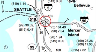
a)

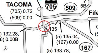
b)

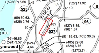
c)

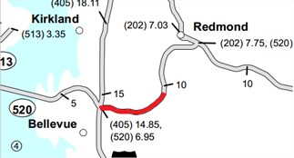
d)

5.2. Open boundary initial random condition

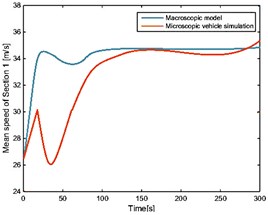
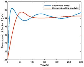
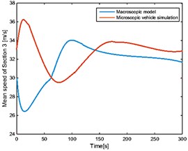
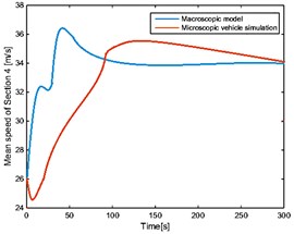
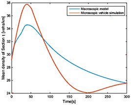
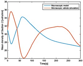
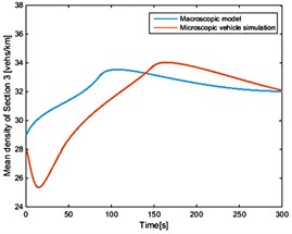
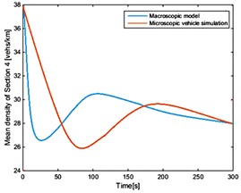
The four sections selected above are considered, using Poisson distribution as starting mechanism and giving speed randomly at 500 meters from the beginning of the road. The speed and position of the automated vehicle at the initial moment are randomly generated. In the open boundary condition with the vehicles entering and leaving the road, and from the macro model and micro simulation, the corresponding characteristic curves are shown in Fig. 2 and Fig. 3 and the corresponding average error is shown in Table 2.

Fig. 2Average velocity of each section of the vehicle under the condition of open boundary random initial conditions

a)

b)

c)

d)

Fig. 3The average density of each section of the vehicle under the condition of open boundary random initial conditions

a)

b)

c)

d)

Table 2The average error of the macro and micro simulation results under the condition of an open boundary steady state

	Section 1	Section 2	Section 3	Section 4
Average velocity	6.27 %	6.67 %	3.01 %	2.23 %
Average density	1.74 %	3.28 %	1.96 %	1.44 %

As shown in Fig. 2 and Fig. 3, vehicle speed and position on the road are generated randomly at the initial time. With the passage of time, automated vehicles gradually adjust their speed to enter the stable state. At the same time, new vehicles are produced in Poisson distribution, which gradually go into the road. These follow the same rules by adjusting their own state to follow the changes in the front car. In the end, all vehicles on the road travel at a steady speed and at the same distance. Due to the effect of the random speed of the starting mechanism, the macro characteristics of each section of the road are simulated by the micro control algorithm. The macroscopic traffic flow model cannot describe the velocity distribution of the microscopic vehicle in detail. Thus, it is unable to reproduce random fluctuations. However, it is consistent with the microscopic simulation of the steady state characteristics and the dynamic evolution trend. As shown in Table 2, the macroscopic characteristics of each section derived from the macro model are basically consistent with the simulation results of the micro control model, and the validity of the model is verified.

5.3. Analysis of the macroscopic traffic model for automated vehicles

In this study, the macroscopic traffic model for automated vehicles will compared with the macroscopic model of the manual driven traffic flow, and the influence of automated vehicles on traffic flow is studied by analyzing the characteristics of speed density and flow density.

Under open boundary conditions, by changing the traffic volume to simulate the different traffic conditions, the velocity - density and volume - density curves of the macroscopic model and the macroscopic manual driven model are as shown in Fig. 4 and Fig. 5.

Fig. 4Macroscopic velocity – density curves under open boundary conditions

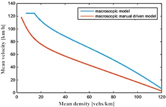
Fig. 5Macroscopic volume – density curves under open boundary conditions

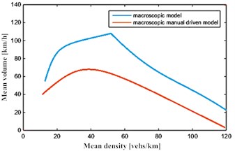
From the simulation curves of Fig. 4, Fig. 5 under open boundary conditions, the traffic velocity-density characteristics and volume-density characteristics of automated vehicles conform to the basic law of traffic flows; and in the same density, the average speed of automated vehicles in traffic and average flow rate are higher than that of the manual driven formation of traffic flow, which can be concluded from Table 3. Taking the open boundary condition as an example, when the density is small, automated vehicle flow and regular vehicle flow are at greater speeds. However, since the density is small, the corresponding traffic volume is small. With the gradual increase in the number of vehicles, the average speed of manual driven traffic is rapidly decreased. However, for automated vehicles, since traffic in the process of moving keeps the driving distance smaller with a faster dynamic response, the traffic rate is obviously higher than that of the manual driving flow (Fig. 4). When the density increases to a certain value, the traffic volume reaches the maximum value. As shown in Fig. 5, the maximum flow rate can be achieved by the automated vehicle flow, which is much higher than the manual driven traffic flow. That is to say, the use of an automated driving system can effectively improve road capacity. With the increase in density, the stop constraints on the road become more and more obvious, the road gradually becomes congested, and the speed and flow rate of automated vehicles and manual driven vehicles are gradually reduced, until it reaches zero. In summary, using automated vehicles can sharply increase the capacity and throughput of roads, and improve its service level, thereby improving traffic.

Table 3The magnitude of improvement of the velocity – density characteristics and volume – density characteristics of the automated traffic flow

	Open boundary condition
Velocity – density characteristic	52.71 %
Volume – density characteristic	69.07 %

5.7. Evaluation of the lane change cooperative

Section 1 is selected to evaluate the impact of the cooperative lane change on the use of intelligent lane changing strategies for the automated vehicle, as shown in Table 5.

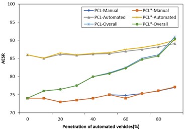
In Fig. 6, PCL/PCL*-Manual/Automated/Overall represents the manual driven car/automated vehicle/mixed car’s AESR with the proportion of the automated driven curve on the off/open channel.

It can be observed that after the opening of the cooperative lane change, with the increase in proportion of automated vehicles, the improvements are huge: manual driven car is not affected, and overall traffic flow efficiency will rise.

In general, collaborative change in driving efficiency on autopilot has a positive impact, but to a certain extent (in automated vehicles, average speed is not used when collaborative lane change increased the maximum of the expected speed to approximately 1 %-2 %); and has no effect on the manual driven car.

Table 5Simulation configuration

Configuration	Value
Lane changing strategy	Intelligent lane changing
Cooperative lane changing	Turn /Off
Expected departure interval	$\lambda :$ 2
Automated vehicle proportion	$\theta$: 0 % $\to$ 100 % 10 %
Lane number	2+3

Fig. 6The chart of AESR

5.8. Effect of the proportion of automated vehicles on traffic flow

Furthermore, the effect of the ratio of automated vehicles on traffic flow under different lane changing coefficients is analyzed. A peak is reached, the traffic flow density is average, the intelligent lane change coefficient is 0.5, and the proportion of automated vehicles to the traffic flow at the selected four sites is simulated, as shown in Table 6.

Table 6Simulation configuration

Configuration	Value
Lane changing strategy	Intelligent lane changing (coefficient of 0.5)
Cooperative lane changing	open
Expected departure interval	$\lambda$: 2, 10
Automated vehicle proportion	$\theta$: 0 % $\to$ 100 %
Lane number	2, 3, 4

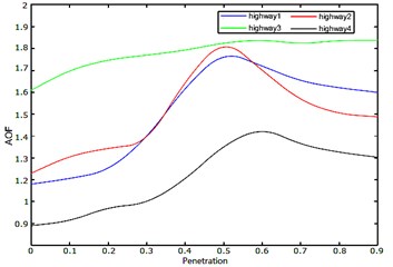
In order to compare the effect of the proportion on traffic volume in the peak/average traffic flow density condition. The comprehensive index of each case ($AOF$) relative to the growth rate of the proportion of automated vehicles is calculated, as shown in Fig. 7, Fig. 8. Based on these results, the proportion of traffic flow improvement can be analyzed.

According to Fig. 7 and Fig. 8, the adoption of automated vehicles induces a significant effect to improve road capacity. When the proportion of automated vehicles on the road increases from 0 % to 10 %, road capacity will increase by 12 %. When the proportion increases to 50 %, road capacity will increase to 56.6 %. When the proportion increases to 90 %, road capacity will go back to 28.3 %. When the proportion falls between 30 % and 40 %, the speed of increasing road capacity is at the greatest. Combined with the traffic conditions of different sections of the road in different periods, we believe that: when the proportion of automated vehicles is near 55 %, the communication capacity of the road is greatly improved. According to the above figures, the adoption of automated vehicles has a significant effect on the improvement of road capacity at the peak traffic hours of crossroads. For roads with lesser lanes, it also has significant effect to improve road capacity. Although automated vehicles slightly sacrifice driving efficiency and bring some impact on the switch reserved distance, the security gained by the road switch strategy covered the shortage of its efficiency. Therefore, efficiency and the security aggregative indicator improved. At the same time, the security and efficiency of automated vehicles obtained a large number of positive impacts, and is indeed a win-win strategy.

Fig. 7The influence of the proportion of automated vehicles on traffic flow during rush hour

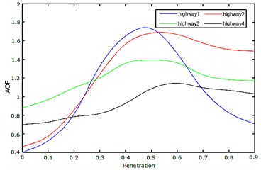
Fig. 8The influence of the proportion of automated vehicles on traffic flow at average density

6. Conclusions

In this study, some models of mixed traffic are presented, which consist of automated vehicles and regular vehicles. By selecting locations randomly, we take the average value of the five cellular automata to the simulating results and validate the reliability of the model in the tolerance.

When the ratio of the automated vehicles in the road is 10 %, the traffic volume of the road is increased, and the capacity of the road is improved slightly. In the interval of 30 %-40 %, the traffic volume is obviously increased, and the road capacity gets the fastest upgrade. When the proportion is about 55 %, road capacity increases mostly obvious. Come to conclusion, the use of automated vehicles has a significant effect on improving the traffic capacity of the congested road section. It is also obvious to enhance the road capacity. In a certain proportion, the traffic capacity of the road is gradually increased, and then gradually decreased.

Each problem discussed above presents an important and very challenging research topic. This paper tried to provide an explicit framework based on macroscopic operational capacity. It’s valuable in both theoretical and practical aspects on modern traffic problems.