Abstract
The vehicle-bridge coupling vibration (VBCV) theory is being applied in the safety evaluation of existing bridges, such as cable-stayed bridge. In order to study the dynamic performance and vibration response of urban long-span cable-stayed bridges under traffic flow, and provide reference for the design, construction and safety assessment of existing bridges, the urban cable-stayed bridge with single tower and double cable in service was taken as the research object. The dynamic response of bridges under vehicles with different number, distance, speed and weight was analyzed. And the VBCV of bridge under different vehicle density and speed was discussed. The traffic flow on the bridge was simulated by the cellular automaton (CA) model, a half car model with four degrees of freedom was established, and the bridge models were established by the ANSYS software. According to the displacement coordination and mechanical balance conditions, the two models were connected, and were solved by MATLAB software. The dynamic response of the vehicle-bridge system under the vehicle fleet and random traffic flow was investigated. The research results showed that the vertical displacement (VD) of the main span increased with the number of vehicles, conversely, the vertical vibration acceleration (VVA) decreased. As driving distance increased, the VD and VVA of main span decreased. The VD of main span was not sensitive to the vehicle speed, but the VVA increased with the vehicle speed. The VD and VVA of the main span increased with the vehicle weight, and the VD of main span was proportional to the traffic density. As the traffic density increased, the VVA increased first, then decreased.
Highlights
- The vertical displacement (VD) increased with the vehicle number under fleet and random traffic flow.
- The vertical vibration acceleration (VVA) was sensitive to the vehicle speed.
- The VD and VVA increased linearly with the vehicle weight.
1. Introduction
Urban cable-stayed bridge plays an important role in the modern transportation. The vehicle-bridge coupling resonance will occur, when the natural vibration frequency of vehicle is close to the first several vibration frequencies of long-span bridge. Therefore, the safety of cable-stayed bridge introduced by the VBCV is an important issue. The VBCV and its factors [1, 2] have been extensively studied. Some studies focused on vehicle bridge model simplification and VBCV analysis methods. Oliva [3] proposed a fully coupled method for reproducing road-vehicle-bridge dynamic interaction. Based on the bridge acceleration response, Domenech [4] adopted a numerical model under the constant moving loads to reproduce the traffic action on the structure. Li [5] proposed a numerical method for stress analysis of railway bridge based on train-bridge coupling dynamics. Deng [6] established the vehicle-bridge coupling equation based on the displacement coordination method. Li [7] calculated the dynamic response of the Fenghua Bridge, and proved that the bridge was safe under the VBCV. Liu [8] obtained the semi-analytical solution of the simply-supported bridge model with moving vehicles. Chang [9] carried out the statistical dynamic analysis on the bridge-vehicle interaction, and obtained the statistical responses, including the mean value and standard deviation of the deflections of beam. Jin [10] investigated the vehicle-bridge interaction effect by considering the damping in the simply-supported bridges. Some studies have investigated vibration under moving vehicles and wind and other excitation sources. Han [11] carried out numerical simulation on the model of Aizhai bridge in China, and obtained the corresponding dynamic stress responses of key parts of the bridge under the combined action of random traffic and wind loads. Wang [12] developed a method identifying vehicle motion parameters, which was used to monitor the bridge deformation and vibration caused by passing vehicles. Rezaiguia [13] studied the response of a multi-span, continuous orthotropic bridge deck under vehicles loads. Hai [14] studied the influence of prestress on the dynamic response of bridge and vehicle. Wang [15] performed a numerical analysis on the dynamic characteristics of multi-span continuous bridges subjected to the interactions of traffic loadings and vehicle dynamic. Gao [16] investigated the dynamic characteristics of the multi-span girder bridge under the moving vehicles. For the random traffic flow, Chen [17] proposed an evaluation method on the vibration comfort considering the randomness of traffic flow. Ho [18] evaluated the dynamic response of a steel box-girder bridge under random traffic flow. Chen [19] studied the live load of a long-span bridge under random traffic. Zhou [20] obtained the dynamic response of each vehicle in random traffic by considering the full-coupling effects for all the vehicles of the traffic flow, bridge and wind.
The above research on the VBCV of bridges is mostly aimed at the highway bridges and the situation of single vehicle passing through bridges. However, the vehicles on urban cable-stayed bridge are mainly small and medium vehicles, which are relatively single and characterized by the random traffic flow. Therefore, the random traffic flow was introduced into the VBCV analysis of urban cable-stayed bridge, which provided a new idea for the VBCV research. The dynamic response of cable-stayed bridge under fleet and random traffic flow was studied, and the influence on the VBCV was analyzed in this study. The vibration response of cable-stayed bridge under different conditions was investigated, including different vehicle number, driving distance, driving speed, vehicle weight, different traffic density and speed, which provided a reference for the future research on the VBCV of cable-stayed bridge and the safety assessment of existing bridges.
2. VBCV model
2.1. CA model parameters
The single lane NaSch (NS) model [21-23] based on cellular automata (CA) was used to simulate the traffic flow. It was a stochastic model in which stochastic deceleration was introduced. The calculation flow of NS model was shown in Fig. 1.
In the Fig. 1, and were the speed of the vehicle (Number ) at the time of and , respectively. was the time step, was the maximum speed on the bridge, was the distance between the vehicle (Number ) and the adjacent vehicle in front. and were the distance to the starting point at the time of and , respectively.
The changes in lane and vehicle types for the urban cable-stayed bridges were not considered, which resulted from the few situations for changing lanes and the relatively uniform vehicle types. Traffic flow was simulated by periodic boundary assumption. It meant that after leaving from the end of the bridge, the vehicle entered from the head of the bridge at the same speed, and continued to cycle during the simulation time. The length of each cell was 1 m, and the maximum speed in the bridge was 22.2 m/s.
The parameters of CA model were listed in Table 1.
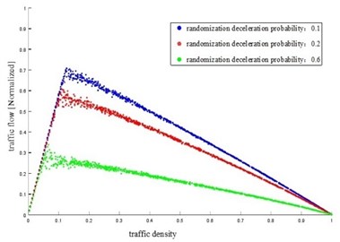
Taking the randomization deceleration probability of the vehicle as a variable, the traffic density with different randomization deceleration probability was obtained, as shown in Fig. 2. Traffic density with different randomization deceleration probability in the reference [24] was shown in Fig. 3.
Fig. 1Calculation flow of NS model
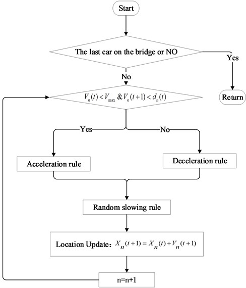
Table 1Parameters of CA model
Parameter | Value |
Section length | 500 m |
Time step | 1 s |
Vehicle length | 5 m |
Speed on road sections | 22 cell/s |
Randomization deceleration probability (Pslow) | 0.1-0.6 |
Figs. 2-3 showed that the traffic flow increased with the traffic density at first, and then decreased. As the randomization deceleration probability increased, the peak value of traffic flow decreased and the road capacity reduced, which was consistent with the actual traffic flow and the results of reference [24]. The CA model established in this paper could reflect the actual traffic flow.
Fig. 2Traffic density with different Pslow of this paper
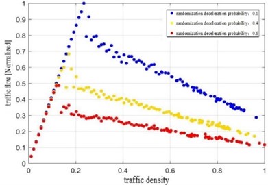
Fig. 3Traffic density with different Pslow of comparative reference
2.2. Vehicle model
A plane model of two-axle vehicle with four degrees of freedom was established by using a semi-vehicle model, as shown in Fig. 4. Pitching degrees of freedom and vibration degrees of freedom were included. The degrees of freedom of the front and rear axles were and . The MASS 21 concentrated mass unit was used to simulate wheels, the COMBIN 14 spring-damper unit was used to simulate the suspension system and the spring-damper system of the wheel. The SHELL 43 unit was used to simulate the vehicle body. The wheel and the car body were connected by a spring damping system.
Fig. 4Plane model of two-axle vehicle
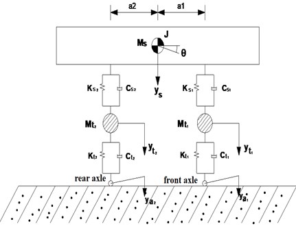
In the Fig. 4, was the mass of vehicle body and frame. , was the mass of front wheel pair and rear wheel pair, respectively. , , and were the vertical connection stiffness and damping coefficient of the air spring, respectively. , , and were the stiffness and damping coefficient of the tire, respectively. , were the distance from the center of the vehicle body to the front and rear wheel pair, respectively. , were the vertical displacement at the contact point of the tire.
The equation of motion of the vehicle was obtained as:
where, was the mass matrix of vehicle. was the damping matrix of vehicle. was the stiffness matrix of vehicle. , , were the VVA, velocity and displacement vectors of vehicles. was the vehicle load vector.
2.3. Engineering example
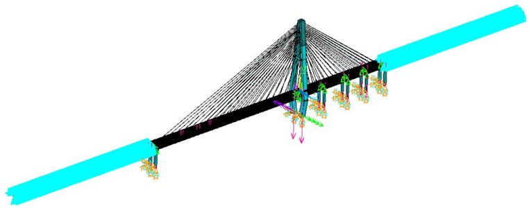
The urban cable-stayed bridge with single tower and double cable in service was taken as the research object. The span of the bridge was 310 m + 50 m + 50 m + 40 m + 40 m. The main span was orthotropic plate steel box girder. The height of the box girder was 3 m and the steel was Q345. The side span was prestressed concrete continuous box girder. The concrete strength grade of the main tower was C50. The height of the main tower above the bridge deck was 126.37 m. The transverse width of the main tower was 4.0 m and the wall thickness was 0.6 m. The longitudinal width of the main tower was 6.0 m and the wall thickness was 1.5 m. There were 37 pairs of stay cables with double cable planes and spatial fan arrangement. The stay cable was a low relaxation galvanized high strength steel wire with a tensile strength standard of 1670 MPa. The design load of the bridge was city-A class, including the dead load of the bridge self-weight and the dynamic load of vehicles. ANSYS was used to build a bridge model. BEAM4 space beam element was used for main beam, main tower, bridge pier and other structures. LINK 10 compression or tension bar element was used for cables of bridge. The spring element was used to simulate the bottom of the pier. The 300 m approach was set up on both sides of the bridge, all the nodes on the approach were constrained. The cable-stayed bridge calculation model was shown in Fig. 5.
Fig. 5Cable-stayed bridge model
The structure was discretized by finite element method. The dynamic differential equation of the bridge was expressed as:
where, was the mass matrix of bridge structure. was the damping matrix of bridge structure. was the stiffness matrix of bridge structure. , , were the vertical acceleration, velocity and displacement vectors of bridge structure. was the bridge structure load vector. The damping of the bridge was Rayleigh damping with viscous damping model, and the damping ratio was 0.03.
Fig. 6Flow chart of VBCV based on ANSYS
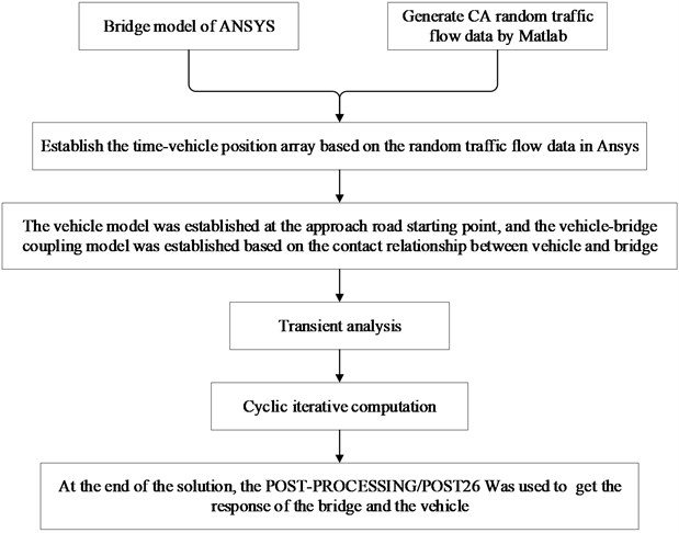
2.4. Solution method of VBCV
The separation method was used to establish the vibration differential equations of vehicles and bridges. The two equations were coupled by displacement compatibility and dynamic equilibrium condition. The MATLAB software was used for programming. The Newmark- gradual integration method was used to solve the equation.
The flow chart of the VBCV based on ANSYS was shown in Fig. 6.
3. Results and discussion
3.1. Vibration response under fleet
The dynamic response of all nodes of the bridge was analyzed by ANSYS software. The dynamic response on the main span of the bridge was the largest, which was 215 m from the main tower, that was, 95 m from the starting point of the bridge. Therefore, this position was taken as the most unfavorable section. The dynamic response was analyzed by controlling the vehicle number, driving distance, driving speed and vehicle weight.
3.1.1. Vehicle number
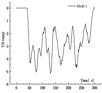
The driving distances between adjacent vehicles in the fleet was set as 40 m, the vehicle weight was 2 t, and the driving speed was 15 m/s. The vehicle number in the fleet was set as 4, 6 and 8, respectively. The VD time history curve and VVA time history curve of the main span of the bridge were obtained, which were shown in Figs. 7-10.
Fig. 7VD time history curve under different vehicles
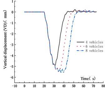
Fig. 8Maximum VD under different vehicles
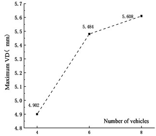
Fig. 9VVA time history curve under different vehicles
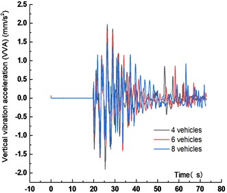
Fig. 10Maximum VVA under different vehicles
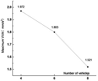
Figs. 7-10 showed that the VD of the main span of the bridge increased with vehicle numbers. When the vehicle number increased from 4 to 6 and 8, the VD increased by 14.4 % and 11.9 %, respectively. The peak time of VD was delayed with the vehicle numbers. The main reason was that with the increase of the vehicle numbers, the distance between the center of gravity of the fleet and the most unfavorable section increased, resulting in the delay of the peak time. The VVA of the bridge decreased with the vehicle numbers. When the vehicle number increased from 4 to 6 and 8, The VVA of the main span was reduced by 8.6 % and 22.9 %, respectively. The main reason was that the increased vehicle numbers made the vehicle bridge interaction influenced each other, which reduced the VVA of the main span.
3.1.2. Driving distance
The vehicle number in the fleet was set as 5, the vehicle weight was 2 t, and the driving speed was 15 m/s. The driving distances between adjacent vehicles in the fleet were 40 m, 60 m and 80 m, respectively. The VD time history curve and VVA time history curve of the main span were obtained, which were shown in Figs. 11-14.
Fig. 11VD time history curve for different driving distances
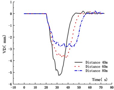
Fig. 12Maximum VD for different driving distances
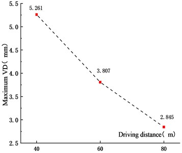
Fig. 13VVA time history curve for different driving distances
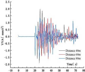
Fig. 14Maximum VVA for different driving distances
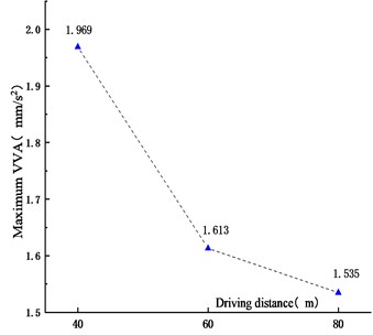
Figs. 11-14 showed that the VD and VVA of the main span decreased with the driving distance. When the driving distances between adjacent vehicles in the fleet increased from 40 m to 60 m and 80 m, the VD reduced by 27.6 % and 45.9 %, and the VVA decreased by 18.1 % and 22.0 %, respectively. This was because that with the increase of the distance between vehicles, the superposition of the VBCV on the unfavorable section was weakened, the VD and VVA of the main span decreased. In addition, due to the increase of driving distance, the length of the fleet increased, resulting in the increase of the time from the center of gravity to the analysis node. The trough time span of the VD time history curve of the main span also increased. In the operation process, the increased driving distance could reduce the VD and VVA of urban cable-stayed bridge effectively, which was beneficial to reduce the bridge vibration and ensure the driving safety of vehicles.
3.1.3. Vehicle speed
The vehicle number in the fleet was set as 7, the vehicle weight was 2 t, and the driving distances between adjacent vehicles in the fleet was 40 m. The vehicle speed was 5 m/s, 10 m/s, 15 m/s and 20 m/s, respectively. The VD time history curve and VVA time history curve of the main span of the bridge were obtained, which were shown in Figs. 15-18.
Fig. 15VD time history curve at different vehicle speed
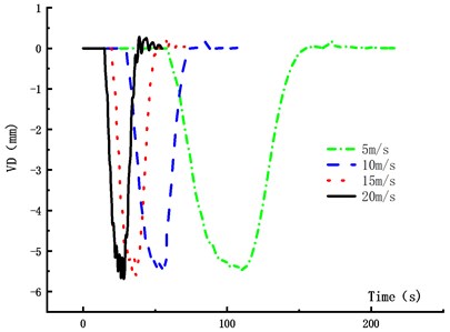
Fig. 16Maximum VD at different vehicle speed
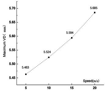
Fig. 17VVA time history curve at different vehicle speed
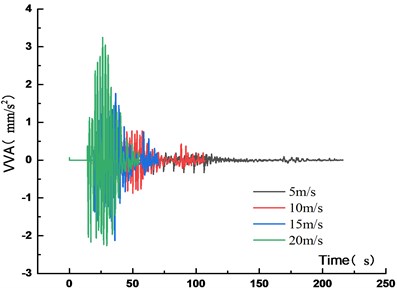
Fig. 18Maximum VVA at different vehicle speed
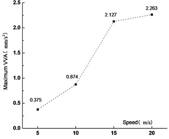
Figs. 15-18 showed that the VD of the main span increased with the vehicle speed. When the vehicle speed increased from 5 m/s to 10 m/s, 15 m/s and 20 m/s, the VD increased by 1.1 %, 2.4 % and 4.1 %, respectively. It showed that the VD of the most unfavorable section was not sensitive to the vehicle speed. With the increased vehicle speed, the passing time of the fleet became short and the running time from the center of gravity to the analysis node was also short, but the VVA of the main span increased. When the vehicle speed increased from 5 m/s to 10 m/s, 15 m/s and 20 m/s, the VVA increased by 133 %, 467 % and 503 %, respectively. It was shown that the VVA of the bridge was sensitive to the vehicle speed. In the operation process, speed control was not only beneficial to traffic safety, but also to the overall structural safety of the bridge.
3.1.4. Vehicle weight
The vehicle number in the fleet was set as 7, the driving distances between adjacent vehicles in the fleet was 40 m and the driving speed was 15 m/s. The vehicle weight was 2 t, 4 t, 6 t and 8 t, respectively. The VD time history curve and VVA time history curve of the main span of the bridge were obtained, as shown in Figs. 19-22.
Fig. 19VD time history curve under different vehicle weights
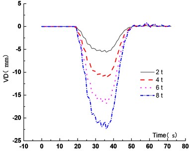
Fig. 20Maximum VD under different vehicle weights
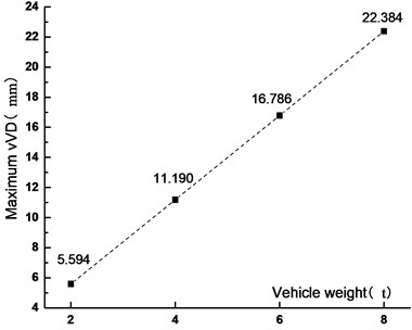
Fig. 21VVA time history curve under different vehicle weights
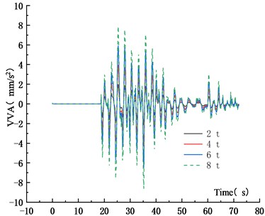
Fig. 22Maximum VVA under different vehicle weights
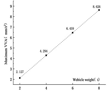
Figs. 19-22 showed that when the vehicle weight increased from 2 t to 4 t, 6 t and 8 t, the VD increased by 100 %, 200.1 % and 300.1 %, respectively. The VD increased linearly. It was shown that the static force played a major role in the VBCV. As the vehicle weight increased, the VVA increased. When the vehicle weight increased from 2 t to 4 t, 6 t and 8 t, the VVA of the main span increased by 101.9 %, 203.7 % and 305.5 %, respectively. The VVA increased linearly. Comprehensive analysis showed that the VD and the VVA were sensitive to the vehicle weight. In the operation process, vehicle weight controlling not only improved the safety of the vehicle, but also ensured the stability of the bridge, which was of great significance to extend the service life of the bridge.
3.2. Vibration response under random traffic flow
Different from the fleet passing the bridge with uniform speed, vehicles accelerated or decelerated in the process of driving, the relationship between vehicles was complex and changeable. The dynamic response of the bridge under the random traffic flow was close to the reality. According to different traffic density and speed, the influence of random traffic flow on VBCV was studied.
3.2.1. Vibration response under different traffic density
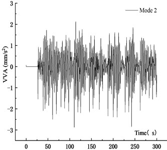
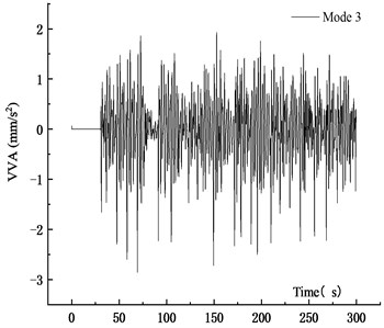
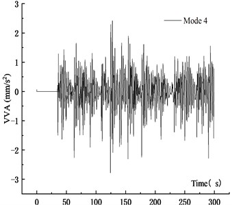
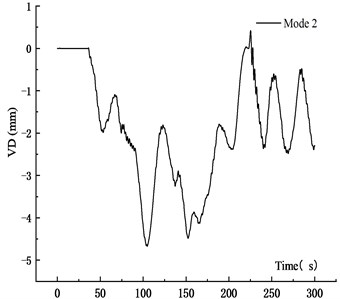
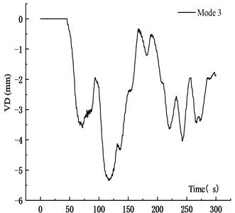
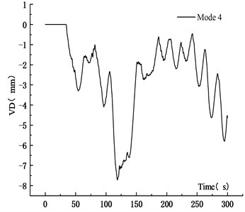
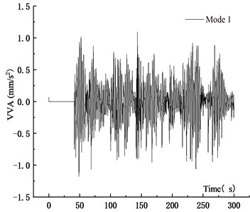
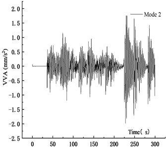
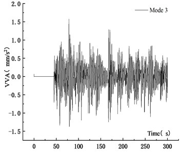
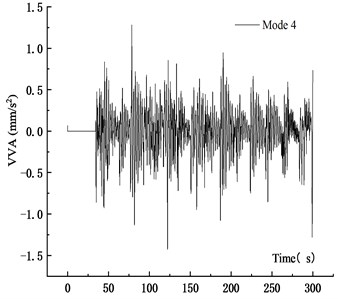
The traffic flow simulated by CA model was set as 9 veh/km (vehicles per kilometer), 20 veh/km and 35 veh/km, corresponding to three operation states of sparse flow, moderate flow and dense flow, respectively. The vehicles were two-axle cars and the traffic flow time was 300 s. To increase the reliability of the simulation, the same traffic density was simulated four times. The simulation results were expressed as mode 1 to mode 4. The random traffic flow under different traffic density was simulated by CA model and was imported into the vehicle-bridge coupling system for analysis. The VD displacement time history curve and VVA time history curve of the main span at 9 veh/km were shown in Figs. 23-24.
Fig. 23VD time history curve at 9 veh/km
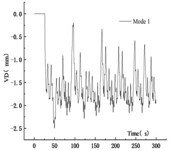
a) Mode 1
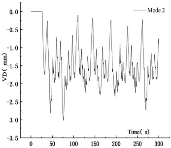
b) Mode 2
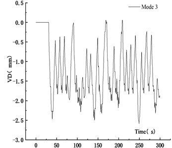
c) Mode 3
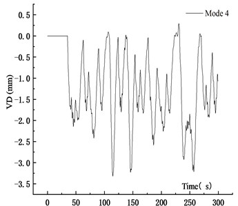
d) Mode 4
Figs. 23-24 showed that the randomness of traffic flow resulted in the vibration curve complex. To reduce the influence of random traffic flow on simulation results, the maximum values under different traffic densities were taken as the average, as listed in Table 2 and Table 3.
Table 2 showed that when the traffic density increased from 9 veh/km to 20 veh/ km and 35 veh/km, the average VD of the main span increased by 113.87 % and 274.68 %, respectively. It showed that the maximum VD of the main span was proportional to the traffic density. Traffic density had a great influence on dynamic deflection. Table 3 showed that as the traffic density increased, the average VVA increased first, then decreased. When the traffic density increased from 9 veh/km to 20 veh/km and 35 veh/km, the average VVA of the main span increased by 17.85 % and 8.30 %, respectively. The main reason was that when the vehicle flow was dense, road congestion occurred. The low speed reduced the VVA of the main span to some extent. Comprehensive analysis showed that the VD of the main span was more sensitive to the change of random traffic density. The increased random traffic density increased the VBCV.
Fig. 24VVA time history curve at 9 veh/km
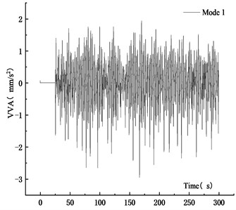
a) Mode 1
b) Mode 2
c) Mode 3
d) Mode 4
Table 2Maximum VD under three traffic densities
Traffic density | Mode | Maximum VD (mm) | Average (mm) |
9 veh/km | 1 | 2.498 | 2.855 |
2 | 3.016 | ||
3 | 2.585 | ||
4 | 3.321 | ||
20 veh/km | 1 | 5.525 | 6.106 |
2 | 5.824 | ||
3 | 6.418 | ||
4 | 6.657 | ||
35 veh/km | 1 | 10.005 | 10.697 |
2 | 13.865 | ||
3 | 11.205 | ||
4 | 7.714 |
Table 3Maximum VVA under three traffic densities
Traffic density | Mode | Maximum VVA (mm/s2) | Average (mm/s2) |
9 veh/km | 1 | 2.961 | 2.868 |
2 | 2.872 | ||
3 | 2.855 | ||
4 | 2.782 | ||
20 veh/km | 1 | 3.586 | 3.380 |
2 | 3.464 | ||
3 | 2.984 | ||
4 | 3.486 | ||
35 veh/km | 1 | 3.833 | 3.106 |
2 | 3.064 | ||
3 | 2.404 | ||
4 | 3.123 |
3.2.2. Vibration response analysis under different speed
The vehicle speed was set as 10 m/s (36 km/h), 15 m/s (54 km/h) and 20 m/s (72 km/h), the traffic density was set as 15 veh/km and the time was 300 s. The influence of random vehicle flow speed on VBCV was analyzed. In order to increase the reliability of the simulation, the same speed was simulated four times. The simulation results were expressed as mode 1 to mode 4. In order to eliminate the interference of the initial state of the traffic flow on the simulation results, the data from 50 s to 300 s were selected to calculate the average speed and standard deviation. The average speed and standard deviation of vehicle flow under different speed were summarized, which were shown in Table 4.
Table 4Statistics of CA simulation traffic flow under different speed
Traffic density | Vehicle speed | Mode | Average speed (m/s) | Standard deviation |
15 veh/km | 10 m/s | 1 | 7.762 | 1.078 |
2 | 7.606 | 1.039 | ||
3 | 7.383 | 0.854 | ||
4 | 7.887 | 0.919 | ||
Average | 7.660 | 0.973 | ||
15 m/s | 1 | 10.814 | 1.562 | |
2 | 11.611 | 1.253 | ||
3 | 11.340 | 1.678 | ||
4 | 11.032 | 1.702 | ||
Average | 11.199 | 1.549 | ||
20 m/s | 1 | 14.873 | 2.108 | |
2 | 14.569 | 2.201 | ||
3 | 15.221 | 1.853 | ||
4 | 15.270 | 1.615 | ||
Average | 14.983 | 1.944 | ||
Table 4 showed that the standard deviation of vehicle average speed increased with the vehicle speed, which indicated that the stability of vehicle speed was weakened, but the overall speed was stable. It was shown that there was no congestion at low traffic density. The vehicle flow data simulated by CA model under different speeds were imported into the VBCV program. The VD time history curve and VVA time history curve of the main span at the speed of 10 m/s were shown in Figs. 25-26.
Figs. 25-26 showed the VD time history curve and VVA time history curve of the main span when the speed was 10 m/s. The maximum values of multiple analysis results under different vehicle speed were averaged to reduce the interference of traffic flow on simulation results. The Maximum VD and VVA at three vehicle speed were showed in Table 5 and Table 6.
Fig. 25VD time history curve at 10 m/s
a) Mode 1
b) Mode 2
c) Mode 3
d) Mode 4
Table 5Maximum VD at three vehicle speed
Vehicle speed | Mode | Maximum VD (mm) | Average (mm) |
10 m/s | 1 | 5.143 | 5.719 |
2 | 4.669 | ||
3 | 5.345 | ||
4 | 7.719 | ||
15 m/s | 1 | 7.943 | 7.458 |
2 | 7.583 | ||
3 | 6.548 | ||
4 | 7.758 | ||
20 m/s | 1 | 9.085 | 8.540 |
2 | 8.370 | ||
3 | 8.877 | ||
4 | 7.828 |
Table 5 showed that when the vehicle speed increased from 10 m/s to 15 m/s and 20 m/s, the average VD of the main span increased by 30.41 % and 49.33 %, respectively. The maximum VD was proportional to the vehicle speed. The main reason was that when the vehicle passed through the bridge quickly, the coupling effect between vehicle and bridge was significant, and the VBCV was obvious. The stability of the average vehicle speed was weakened, which affected the VBCV. Therefore, the increased deflection of the speed from 10 m/s to 15 m/s was greater than that from 15 m/s to 20 m/s. Table 6 showed that the VVA of the main section increased with the speed. When the vehicle speed increased from 10 m/s to 15 m/s and 20 m/s, the average VVA of the main span increased by 75.41 % and 193.71 %, respectively. It showed that the VVA of the bridge was more sensitive to the vehicle speed. Comprehensive analysis showed that the VBCV at high speed was greater than that at low speed obviously.
Table 6Maximum VVA at three vehicle speed
Vehicle speed | Mode | Maximum VVA (mm/s2) | Average (mm/s2) |
10 m/s | 1 | 1.177 | 1.541 |
2 | 1.985 | ||
3 | 1.576 | ||
4 | 1.427 | ||
15 m/s | 1 | 2.803 | 2.703 |
2 | 2.660 | ||
3 | 2.647 | ||
4 | 2.703 | ||
20 m/s | 1 | 3.787 | 4.526 |
2 | 4.748 | ||
3 | 5.516 | ||
4 | 4.054 |
Fig. 26VVA time history curve at 10 m/s
a) Mode 1
b) Mode 2
c) Mode 3
d) Mode 4
4. Conclusions
The urban cable-stayed bridge with single tower and double cable in service was taken as the research object. The vehicle bridge coupling model was established under fleet and random traffic flow. The dynamic response of bridges under vehicles with different number, distance, speed and weight was analyzed. And the VBCV of bridge under different vehicle density and speed was discussed. Some important conclusions can be summarized as follows:
1) The VD of VBCV increased significantly with the vehicle number under fleet and random traffic flow. As the vehicle number increased under fleet, the VVA decreased, but as the traffic density increased under the random traffic flow, the VVA increased first, then decreased. The interaction between vehicle and bridge was influenced by the increased vehicle number and the VVA of the main section was reduced. High traffic density resulted in low speed under random traffic flow, and the comprehensive effects of vehicle speed and traffic density would reduce the VVA of the bridge.
2) The vibration of the bridge increased with the vehicle speed, and VVA of the bridge was sensitive to the vehicle speed. When the vehicle speed increased from 10 m/s to 15 m/s and 20 m/s, the average VVA increased by 75.41 % and 193.71 %, respectively. The vehicle speed was a major factor in the VBCV.
3) As driving distance increased, the VD and VVA of the main span decreased. When the driving distance increased from 40 m to 60 m and 80 m, the VD reduced by 27.6 % and 45.9 %, and the VVA decreased by 18.1 % and 22 %, respectively.
4) When the vehicle weight increased from 2 t to 4 t, 6 t and 8 t, the VD of the main span increased by 100.0 %, 200.1 % and 300.1 % and the VVA increased by 101.9 %, 203.7 % and 305.5 %, respectively. The VD and VVA increased linearly with the vehicle weight, and the vehicle weight had a great influence on the bridge vibration.
References
-
W. Wang, W. Yan, L. Deng, and H. Kang, “Dynamic analysis of a cable-stayed concrete-filled steel tube arch bridge under vehicle loading,” Journal of Bridge Engineering, Vol. 20, No. 5, p. 04014082, May 2015, https://doi.org/10.1061/(asce)be.1943-5592.0000675
-
J.-G. Zhou and G.-H. Wang, “Coupling vibration research on vehicle-bridge system,” IOP Conference Series: Earth and Environmental Science, Vol. 267, No. 4, p. 042104, Jun. 2019, https://doi.org/10.1088/1755-1315/267/4/042104
-
J. Oliva, J. M. Goicolea, P. Antolín, and M. Astiz, “Relevance of a complete road surface description in vehicle-bridge interaction dynamics,” Engineering Structures, Vol. 56, pp. 466–476, Nov. 2013, https://doi.org/10.1016/j.engstruct.2013.05.029
-
A. Doménech, P. Museros, and M. D. Martínez-Rodrigo, “Influence of the vehicle model on the prediction of the maximum bending response of simply-supported bridges under high-speed railway traffic,” Engineering Structures, Vol. 72, pp. 123–139, Aug. 2014, https://doi.org/10.1016/j.engstruct.2014.04.037
-
H. Li, H. Xia, M. Soliman, and D. M. Frangopol, “Bridge stress calculation based on the dynamic response of coupled train-bridge system,” Engineering Structures, Vol. 99, No. 15, pp. 334–345, Sep. 2015, https://doi.org/10.1016/j.engstruct.2015.04.014
-
L. Deng and C. S. Cai, “Identification of dynamic vehicular axle loads: demonstration by a field study,” Journal of Vibration and Control, Vol. 17, No. 2, pp. 183–195, Feb. 2011, https://doi.org/10.1177/1077546309351222
-
Z. L. Li, P. Y. Zhou, and Z. B. Yun, “Study on the vehicle-bridge coupling vibration of steel arch bridge,” Advanced Materials Research, Vol. 163-167, pp. 233–238, Dec. 2010, https://doi.org/10.4028/www.scientific.net/amr.163-167.233
-
X.-W. Liu, J. Xie, C. Wu, and X.-C. Huang, “Semi-analytical solution of vehicle-bridge interaction on transient jump of wheel,” Engineering Structures, Vol. 30, No. 9, pp. 2401–2412, Sep. 2008, https://doi.org/10.1016/j.engstruct.2008.01.007
-
T.-P. Chang, “Stochastic dynamic finite element analysis of bridge-vehicle system subjected to random material properties and loadings,” Applied Mathematics and Computation, Vol. 242, pp. 20–35, Sep. 2014, https://doi.org/10.1016/j.amc.2014.05.038
-
Z. Jin, B. Huang, S. Pei, and Y. Zhang, “Energy-based additional damping on bridges to account for vehicle-bridge interaction,” Engineering Structures, Vol. 229, p. 111637, Feb. 2021, https://doi.org/10.1016/j.engstruct.2020.111637
-
Y. Han, K. Li, C. S. Cai, L. Wang, and G. Xu, “Fatigue reliability assessment of long-span steel-truss suspension bridges under the combined action of random traffic and wind loads,” Journal of Bridge Engineering, Vol. 25, No. 3, p. 04020003, Mar. 2020, https://doi.org/10.1061/(asce)be.1943-5592.0001525
-
H. Wang, T. Nagayama, B. Zhao, and D. Su, “Identification of moving vehicle parameters using bridge responses and estimated bridge pavement roughness,” Engineering Structures, Vol. 153, pp. 57–70, Dec. 2017, https://doi.org/10.1016/j.engstruct.2017.10.006
-
A. Rezaiguia, N. Ouelaa, D. F. Laefer, and S. Guenfoud, “Dynamic amplification of a multi-span, continuous orthotropic bridge deck under vehicular movement,” Engineering Structures, Vol. 100, pp. 718–730, Oct. 2015, https://doi.org/10.1016/j.engstruct.2015.06.044
-
H. Zhong, M. Yang, and Z. J. Gao, “Dynamic responses of prestressed bridge and vehicle through bridge-vehicle interaction analysis,” Engineering Structures, Vol. 87, No. 15, pp. 116–125, Mar. 2015, https://doi.org/10.1016/j.engstruct.2015.01.019
-
L. Wang, X. Kang, and P. Jiang, “Vibration analysis of a multi-span continuous bridge subject to complex traffic loading and vehicle dynamic interaction,” KSCE Journal of Civil Engineering, Vol. 20, No. 1, pp. 323–332, Jan. 2016, https://doi.org/10.1007/s12205-015-0358-4
-
Q.-F. Gao, Z.-L. Wang, C.-G. Liu, J. Li, H.-Y. Jia, and J.-F. Zhong, “Dynamic responses of a three-span continuous girder bridge with variable cross-section based on vehicle-bridge coupled vibration analysis,” The IES Journal Part A: Civil and Structural Engineering, Vol. 8, No. 2, pp. 121–130, Apr. 2015, https://doi.org/10.1080/19373260.2015.1014297
-
B. Chen, D. Wu, X. Xie, and P. Lu, “Comfort assessment for a pedestrian passageway suspended under a girder bridge with random traffic flows,” Advances in Structural Engineering, Vol. 20, No. 2, pp. 225–234, Feb. 2017, https://doi.org/10.1177/1369433216660007
-
H. Ho and M. Nishio, “Evaluation of dynamic responses of bridges considering traffic flow and surface roughness,” Engineering Structures, Vol. 225, p. 111256, Dec. 2020, https://doi.org/10.1016/j.engstruct.2020.111256
-
S. R. Chen and J. Wu, “Modeling stochastic live load for long-span bridge based on microscopic traffic flow simulation,” Computers and Structures, Vol. 89, No. 9-10, pp. 813–824, May 2011, https://doi.org/10.1016/j.compstruc.2010.12.017
-
Y. Zhou and S. Chen, “Fully coupled driving safety analysis of moving traffic on long-span bridges subjected to crosswind,” Journal of Wind Engineering and Industrial Aerodynamics, Vol. 143, pp. 1–18, Aug. 2015, https://doi.org/10.1016/j.jweia.2015.04.015
-
Lu Xiaojun et al., “Research on simulation method of long-span bridge traffic load based on CA model,” China and Foreign Highway, Vol. 33, No. 6, pp. 89–93, 2013.
-
Liu Yingdong, “Cellular automata simulation of urban road traffic flow based on deceleration effect,” Lanzhou Jiaotong University, Lanzhou, 2016.
-
Ruan Xin et al., “Bridge traffic flow synthesis and load simulation based on multi-cell model,” Journal of Tongji University (Natural Science Edition), Vol. 7, pp. 5–11, 2017.
-
Wu Mengchang, “Vehicle-bridge coupled vibration analysis of highway bridge based on random traffic flow,” Huazhong University of Science and Technology, Wuhan, 2018.
Cited by
About this article

The authors would like to gratefully acknowledge the financial support from Tianjin Natural Science Foundation (Nos. 17JCYBJC22300, 17JCZDJC31800, 18JCQNJC08300, 18JCYBJC90800), Tianjin transportation Science and Technology Development Plan (2021-20), Key Laboratory of Road Structure and Materials Transportation Industry (No. 310821171114), Innovation capability support plan of Shaanxi Province (No. 2019KJXX-036), Scientific Research Project of Tianjin Education Commission (No. 2020KJ038), Department of Science and Technology of Shaanxi Province Focuses on Research and Development of General Project Industrial Field (No. 2020GY318), and National Natural Science Foundation of China (No. 52108333).
