On the use of signal smoothness estimates and signal similarity in bearing fault detection

1. Introduction

The rolling bearing is one of the most important and widely used components in various mechanical units and mechanisms. Unexpected fault of the item can cause significant material damage, interrupting the units work. Defective bearing often leads out of a stable rotational axis of the rotor, then a chain reaction of faults can occur throughout the unit. To avoid such accidents, it is highly important to identify the bearing defect at the earliest stage. That is why the diagnostic methods of bearing defects have been intensively investigated in recent years. Vibro-acoustic signals are often used in the condition monitoring and preventive maintenance of the rolling bearing [1].

In this study, a new fault bearing feature extraction method based on signal smoothness and signal similarity estimates is proposed.

The organization of the rest of this paper is as follows: Section 2 reviews the notions and mathematical interpretation of signal smoothness and signal similarity. The basic defect detection principles are introduced in Section 3. Section 4 gives some experimental analysis results. Finally, some conclusions are drawn in Section 5.

2. Signal smoothness and signal similarity: mathematical interpretation

The notion of smoothness of a digital vibro-acoustic signal $X=\left(X\right(0\left)\mathrm{}\mathrm{}X\right(1)\mathrm{}\mathrm{}\dots \mathrm{}\mathrm{}X(N-1){)}^T$$(N=2^n,$$n\in \mathbb{N})$ is introduced in a spectral domain, i.e. the original signal $X$, first and foremost, is subjected to an arbitrary discrete transform (Fourier, Cosine, Walsh-Hadamard, etc.). It is well known that any discrete transform (DT) is uniquely specified by its matrix $T$, namely:

here: $Y$ is the DT spectrum of $X$ and $T$ is the DT matrix. If the DT basis vectors (rows of the matrix $T$) are represented in a frequency order, then the spectral coefficients $Y\left(k\right)$ ($k\in \left\{0,1,\dots ,N-1\right\}$) have tendency to decrease in absolute value, as their serial numbers $k$ increase. So, the array of coefficients $\left\{\left.\left|Y\left(k\right)\right|\right|k=1,\mathrm{}2,\dots ,\mathrm{}N-1\right\}$ can be approximated by a hyperbolic curve $y=C/x^{\alpha }$, where $C\ge 0$ and $\alpha \ge 0$.

The quantity $\alpha$, characterizing the shape of the hyperbolic curve, i.e. the rate of “decay” of spectral coefficients is assumed to be the smoothness parameter (level, class) of the signal $X$.

In this paper, we explore the discrete cosine transform (DCT), because this transform distinguishes itself with very good signal energy “compaction” (at lower frequencies) property [2].

In particular, the DCT matrix $T$ comprises elements:

for all $m=\mathrm{0,1},\dots ,N-1$ and $k=\mathrm{1,2},\dots ,N-1$.

For more details (computational procedures, two-dimensional case), you can refer to [3].

To introduce the concept of signal similarity, we here take two arbitrary fragments of the vibro-acoustic signal $X$, namely: $U=\left(U\right(0\left)\mathrm{}\mathrm{}U\right(1)\mathrm{}\mathrm{}\dots \mathrm{}\mathrm{}U(M-1){)}^T$$(M<N)$ and $V=U+∆U$, where $∆U$ is a small increment assigned to $U$. Let ${\alpha }_U$ and ${\alpha }_V$ signify smoothness parameter values (estimates) of $U$ and $V$, respectively.

For assessing the fragmental similarity between $U$ and $V$, the mean squared error (metrics) $\delta$ is used, i.e.

The vibro-acoustic signals (fragments) $U$ and $V$ are said to be similar if $\delta =\delta (U,V)\le {\delta }_0$ (${\delta }_0$ being a priori fixed positive number).

It has been proved [4] that small changes in some values of the fragment $U$ led to small changes in the smoothness parameter value ${\alpha }_U$, i.e.:

where ${\epsilon }_0$ depends on ${\delta }_0$.

Consequently, the precondition for non-similarity of signal fragments $U$ and $V$ is defined by the following relationship (the necessary condition for fragmental similarity):

In other words, signal fragments $U$ and $V$ cannot be similar if their smoothness parameter values differ significantly (in the mean squared error sense).

3. The general bearing fault detection idea

To describe the potential capability and effectiveness of application of both the signal smoothness estimates and the signal similarity to vibro-acoustic signal defect detection process, the following considerations have been taken into account:

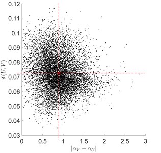
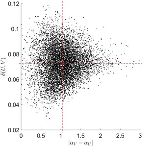
(1) The original signal (rolling bearing signal under normal conditions) $X=\left(X\right(0\left)\mathrm{}\mathrm{}X\right(1)\mathrm{}\mathrm{}\dots \mathrm{}\mathrm{}X(N-1){)}^T$$(N=2^n,$$n\in \mathbb{N})$ is divided into a finite number of non-overlapping fragments $U$ of equal size $2^l$ ($l<n$). For each fragment $U$, the smoothness parameter value (estimate) ${\alpha }_U$ is found. Then, all possible fragments $V$ (of double or triple size, in comparison with $U$) of the same signal $X$ are processed, i.e. their smoothness estimates ${\alpha }_V$ are computed. Finally, for each fragment $U$ (there are $2^{n-l}$ fragments, in total), a plot of points (a “cloud”) $\left\{\left(\left|{\alpha }_U-{\alpha }_V\right|,\delta \left(U,V\right)\right)\right\}$ is determined, and the centre $\left({\left|{\alpha }_U-{\alpha }_V\right|}_{av.},{\delta }_{av.}\left(U,V\right)\right)$ of the “cloud” is found.

(2) By using all the obtained centres $\left({\left|{\alpha }_U-{\alpha }_V\right|}_{av.},{\delta }_{av.}\left(U,V\right)\right)$, the bearing fault detection criterion domain $\mathcal{B}$ is formed, namely:

(3) For the (rolling bearing) test signal $X_{test}$, precisely the same computational steps are performed. The only difference, fragments $U$ are taken from the original signal $X$ and compared with larger fragments $V_{test}$ derived from the signal $X_{test}$.

If a priori prescribed percentage (usually, established experimentally) of centre points $\left({\left|{\alpha }_U-{\alpha }_{V_{test}}\right|}_{av.},{\delta }_{av.}\left(U,V_{test}\right)\right)$ fall into the criterion domain (rectangle) $\mathcal{B}$ (Eq. (6)), then the test signal $X_{test}$ indicates “no fault”, and otherwise (too many centres escape the domain $\mathcal{B}$), the rolling bearing fault is detected.

4. Experimental analysis results

To corroborate the proposed theoretical ideas, a few rolling bearing (vibro-acoustic) signals of size 8192 have been analysed. The test bearing data, i.e. fault diameters (0.1778 mm), frequency (12000 Hz), shaft rotating speed of the motor (1772 rpm) and the signals themselves were obtained from the Bearing Data Center of Case Western Reserve University [5].

The rolling bearing signal $X$ under normal conditions is presented in Fig. 1, and the rolling bearing signals under ball fault, inner race fault and outer race fault conditions are shown in Fig. 2.

Fig. 1Vibro-acoustic signal X of size 8192, under normal condition

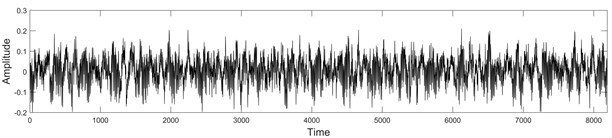
Fig. 2Vibro-acoustic signals Xtest of size 8192, under fault conditions

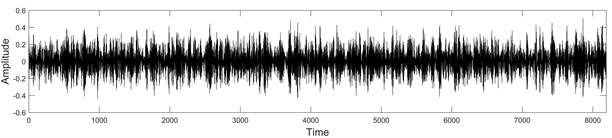
a) Ball fault condition

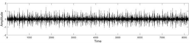
b) Inner race fault condition

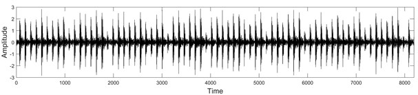
c) Outer race fault condition

First of all, the defect detection criterion domain $\mathcal{B}$ was found out, that it is: $\mathcal{B}=\left\{\left.\left(\left|{\alpha }_U-{\alpha }_V\right|,\delta \left(U,V\right)\right)\right|0.296\le \left|{\alpha }_U-{\alpha }_V\right|\le 2.009;0.048\le \delta \left(U,V\right)\le 0.101\right\}$ (Fig. 3). Then for each fragment $U$ ($\left|U\right|=16$), of the vibro-acoustic signal $X$, all possible pairings with double-sized fragments $V$ of the test signal $X_{test}$ (Fig. 2) have been examined.

Fig. 3The formation of the rectangular domain B of signal defect detection criterion

In Fig. 4-Fig. 6, both the criterion domain (rectangle) $\mathcal{B}$ and some typical situations, with earlier-mentioned centre points $\left({\left|{\alpha }_U-{\alpha }_{V_{test}}\right|}_{av.},{\delta }_{av.}\left(U,V_{test}\right)\right)$ escaping the domain $\mathcal{B}$, are shown.

Fig. 4Typical rolling bearing signal fragments under ball fault conditions

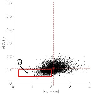
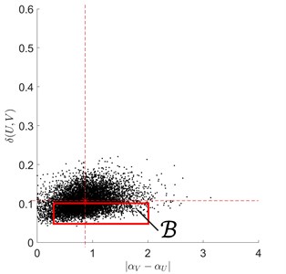
Fig. 5Typical rolling bearing signal fragments under inner race fault conditions

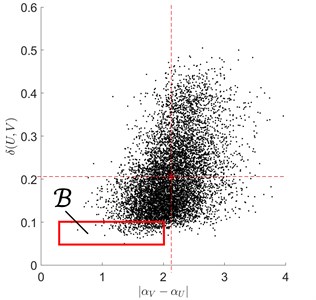
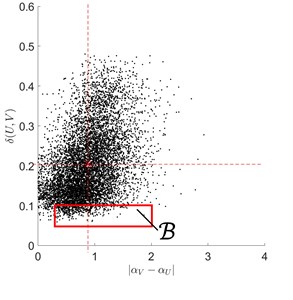
Fig. 6Typical rolling bearing signal fragments under outer race fault conditions

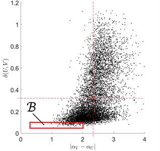
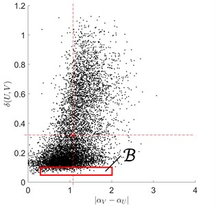
We here note, that: in the case of $X_{test}$ under ball fault conditions, 58 % of centre points escaped $\mathcal{B}$; in the case of $X_{test}$ under inner and outer race fault conditions, all centre points (i.e. 100 %) escaped $\mathcal{B}$.

Often, for practical applications, to minimize computational time expenditure, the necessary signal similarity condition (Eq. (5)) is employed, i.e. in the general bearing fault detection steps, only pairings $U\leftrightarrow V$, with $\left|{\alpha }_U-{\alpha }_V\right|\le {\epsilon }_0$ (${\epsilon }_0$ being a priori prescribed positive number) are analysed.

5. Conclusions

This paper presents mathematical interpretation of fragmentary smoothness and similarity of vibro-acoustic signals. The smoothness of the signal is assumed to be a real number characterizing the downtrend of the spectral DT coefficients, as their serial numbers increase.

The main attention is paid to a newly developed vibro-acoustic signal defect detection technique based on the use of signal smoothness and signal similarity estimates.

Preliminary experimental analysis results showed that the proposed technique was sensitive enough to detect abnormal conditions in the rolling bearing signal.

References

-
Luo G. Y., Osypiw D., Irle M. Real-time condition monitoring by significant and natural frequencies analysis of vibration signal with wavelet filter and autocorrelation enhancement. Journal of Sound and Vibration, Vol. 236, Issue 3, 2000, p. 413-430.
Hsu C. T., Wu J. L. Energy compaction capability of DCT and DHT with CT image constraints. Proceedings of the International Conference on Digital Image Processing, 1997, p. 345-358.
Žumbakis T., Valantinas J. Definition, evaluation and task-oriented application of image smoothness estimates. Information Technology and Control, Vol. 2, Issue 31, 2004, p. 16-23.
Vaideliene G., Valantinas J. On the detection of self-similarities in vibro-acoustic signals. Journal of Vibroengineering, Vol. 17, Issue 8, 2015, p. 4259-4267.
Bearing Data Center. Case Western Reserve University, https://csegroups.case.edu/bearing datacenter/pages/download-data-file.
About this article