Abstract
This study outlines the experimental investigation methods of condition monitoring to predict bearing failures using the experimental vibration signatures. The purpose of condition monitoring is to maximize the machine availability and utility of the machine components. Bearings being one of the most common component in any rotating machinery, it is vital to study the health of the bearing and can predict bearing failure, its location and severity. This prevents machine downtime, monetary loss and unfortunate accidents. A test rig was fabricated to get the vibration signatures of bearings. Prediction of bearing failure relies on the presence of the bearing characteristic frequencies – inner race frequency, outer race frequency, ball pass frequency and fundamental train frequency – and its harmonics in the vibration signal acquired. These frequencies are present in the vibration signature due to the interaction of surfaces of different bearing components that have defects in them. Both time and frequency domain numerical signature analysis were performed on the vibration signatures acquired. Simple frequency domain method like Fast Fourier Transform (FFT), chaotic vibration method like modified Poincare mapping and time-frequency domain Wigner-Ville distribution (WVD) were used in detecting bearing failure. Using the FFT analysis method, it is hard to predict the failures, hence better signal processing methods like modified Poincare mapping and WVD are used. Also, it is observed that the chaotic vibration signatures found in the lower-order mechanical systems like bearings. With the chaotic analysis methods like, Poincare Mapping and Wigner-Ville Distribution, the location and the severity of the bearing failure can be predicted.
1. Introduction
The philosophy of machine condition monitoring is to monitor the state of the machine and to detect any deterioration in condition, to determine the cause of the failure and to predict the expected time of failure. So, Machine condition monitoring deals with the maintenance aspects of the machines based on the present and past condition of the machine. For the assessment of the condition of the machine, sensors are installed on and / or around the machine to get the data like vibration amplitude, acoustic emission etc. This data is analysed based on experience and standards of fault diagnosis and decisions are taken regarding maintenance or corrective actions. The result is to maximize machine availability and utility of the machine elements like bearings, gears, etc. to the fullest.
Lubricant analysis [3], acoustic emission, vibration analysis and diagnostics [2], infrared thermography [4], ultrasound testing (Material Thickness/Flaw Testing) and motor condition monitoring and motor current signature analysis (MCSA) are few condition monitoring techniques applied in the industrial and transportation sectors. Most condition monitoring technologies are being slowly standardized by ASTM and ISO [5].
The most commonly used method for rotating machines is vibration analysis. In rotating machinery, detection of fatigue failure is an important problem. The result of not detecting a failure in time would be severe damage to machinery, catastrophic injuries, and substantial financial loss.
Even small defects like surface roughness and scratch can be detected using vibration signatures. The vibration signals are complicated by the interaction of the various component parts, but this can be often used to advantage, to detect a deterioration or damage to the rolling surfaces. This interaction of the imperfections on the surface of raceways and rolling elements produce four discrete characteristic frequencies and their sidebands – Ball Pass Frequency for Inner Race (BPFI), Ball Pass Frequency for Outer Race (BPFO), Fundamental Train Frequency (FTF) and Ball Pass Frequency (BPF). Analysis of vibration signals is usually complex and the characteristic frequencies generated will add and/or subtract and are almost always present in the vibration spectra. This is particularly true where multiple defects are present.
However, bearing frequencies can be difficult to detect in the early stage of a defect because of the dynamic range of the equipment, background noise level and other sources of vibration. Over the years several diagnostic algorithms have been developed to detect bearing faults by measuring the vibration signatures on the bearing housing.
Numerical vibration signature analysis methods like Fast Fourier Transform (FFT) works in frequency domain, modified Poincare mapping works in time domain and Wigner-Ville Distribution (WVD) works in both time and frequency domain. The joint time-frequency distribution provides an interactive relationship between time and frequency during the time interval of data window, and detect the damage of elements. These methods include Short Time Fourier Transform (STFT), Wigner-Ville Distribution (WVD), Wavelet Transform (WT), Choi-Williams Distribution and Hyper Coherence Function, etc. In this paper, we are using the Wigner-Ville Distribution method to provide good resolution along both time and frequency scales for the vibration signals in comparison with other joint time-frequency transforms. To examine the vibration signal, joint time-frequency analysis method was chosen to provide an instantaneous frequency spectrum of the system at every instant of the revolution of the shaft, while a Fourier Transform can only provide the average vibration spectrum of the signal obtained during one complete revolution. In other words, the time-changing spectral density from the joint time-frequency spectra will provide information concerning the frequency distribution concentrated at that instant around the excited instantaneous frequency which cannot be obtained in a regular vibration frequency spectrum. The WVD is a real-valued function of time and frequency, i.e. the WVD can be viewed as an image or a matrix. [6] The WVD of the signal has a significant change in the energy distribution at the location where the vibration signal amplitude decreases. This decrease results in the decrease of the signal energy, which was displayed by the lighter shades of the WVD image.
The application of chaotic method in identifying and quantifying ball bearing damage had not been fully investigated. The use of chaotic vibration analysis had been first performed by Ehrich [1, 7]. Several authors introduced chaotic method to process signals [8-12]. In the modified Poincare map [13] using the shaft speed, each position of shaft motion from 0° to 360° is generated. A series of Poincare maps is obtained for every shaft position and then used to construct the modified Poincare Map for shaft rotational speed. The modified Poincare map for the relative carrier speed is generated in a similar way with the vibration data obtained from a complete revolution based on the relative carrier speed. Normalizing vibration amplitudes in both and directions, a modified Poincare map of the vibration signals can be constructed. The vibrations resulted from the bearing race damage can generally be expressed in some repeatable fashions using the repeatable time that the rolling element passes over the damaged area. However, due to the chaotic motion i.e. changing rotational direction of the ball elements, the vibrations resulted from the ball element surface damage is general chaotic and non-repeatable. In this paper, we are proposing to use all these three methods for fault detection from the analysis of the vibration signature obtained from an experimental setup.
2. Vibration signature analysis
Vibration signature analysis methods for condition monitoring have become the advanced fault identification procedures. They are used in rotating mechanical systems to fulfil the increasing requirements for safe operation and long life in mechanical systems.
To construct a methodology to predict the bearing failure, a thorough understanding of the vibration signal of the bearing setup is necessary. Vibration signal analysis methods like FFT, WVD and Poincare mapping are performed on the acquired vibration signature. These methods can be classified into frequency domain analysis, joint time-frequency domain analysis and chaotic methods respectively. Comparison of the vibration signatures obtained with a signature data bank of the healthy machine allow the detection of defect in the bearing. This process does not require the rotating machinery to be shut down, and is now being used as an on-line diagnostic and trend monitoring tool [5].
2.1. Fast Fourier Transform (FFT)
An appropriate signal processing method can easily detect changes in the vibration signal caused by the fault in the bearing components. Traditional analysis has relied on spectrum analysis like Fast Fourier Transform (FFT). FFT transforms a vibration signal from time based domain to frequency domain. [14] Henceforth, giving us the frequency spectrum that includes all the signal’s fundamental frequency and its harmonics:
where is time domain response of any system, is Fourier Transform of .
In this algorithm, the assumption is, within a single time interval, the frequency change is small, such that there is no violation of the necessity of a stationary signal for frequency transformation. If the frequency change is significant within this time interval, then the FFT will yield an error in the actual value of the signal.
FFT is easy to implement and the most common vibration signal processing tool. However, this method does not give us information about the time dependence of the vibration signal being analysed, as the FFT results are averaged over the signal’s time duration. This becomes a problem when analysing non-stationary signals. It is often beneficial to acquire a correlation between the time and frequency contents of the signal in such cases. FFT analysis is thus not suitable for the detection of the bearing characteristics, which are an important part of the vibration signature. Hence, more powerful signal processing methods are needed to unambiguously detect all faults [15].
2.2. Wigner-Ville distribution (WVD)
The limitation of the FFT mentioned in Section 2.1 has led to the introduction of joint time-frequency signal processing methods, such as the Wigner-Ville Distribution (WVD), Short-Time Fourier Transform (STFT) [16] and others. These methods map a signal into a two- dimensional (2D) function of time and frequency.
WVD is a good analysis method because of its good time and frequency resolution. WVD allows an accurate description of spectral events associated with fast changes in the bearing vibration signature. However, the WVD present difficulties due to the presence of interference terms when dealing with multi-component signals [17, 18]. Taking into consideration the characteristics of bearing signature in the selection of the analysis and time smoothing windows, smoothing the WVD, alleviates this problem and allows the extraction of important cues on the time-frequency plane [19]. The WVD in discrete form can be defined as:
where is the Wigner-Ville distribution in both the time domain and frequency domain , is the time signal, is the sampling period, and is the length of time data used in the transform. The quadratic operation on the signal causes the WVD to be a bilinear transformation. For a composite signal :
The third term in the above equation is known as a cross-term. It is due to the interference between the two components. A cross-term appears midway between the two components and oscillates in time, at a rate equal to the frequency separation between them. Its amplitude is proportional to the product of the two components’ amplitudes. To avoid this aliasing problem arising in the computation of the WVD, the original real signal is transformed into a complex analytic signal. It also reduces the bandwidth to one half, thus avoiding double Nyquist rate sampling which is required for a real signal. The analytic signal is obtained by adding the signal’s Hilbert transform , as it’s imaginary part or by using its definition in the frequency domain. The WVDs of the analytic and real signal are related by:
where, .
The window length limits the accuracy of extracting frequency information relative to the duration of the signal. The area (time bandwidth product) of the window function in the time-frequency plane remains fixed once the window function is defined, which means that the time and frequency resolutions cannot be increased simultaneously.
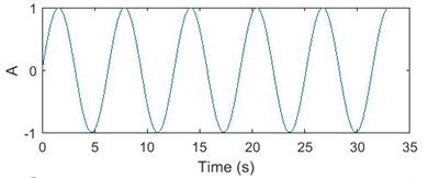
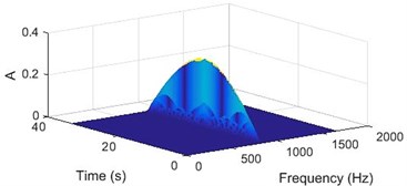
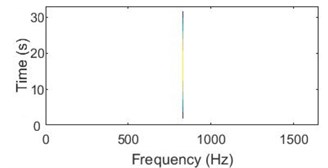
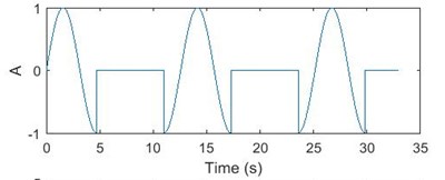
This method can be used to examine a time domain signal and provide an instantaneous frequency spectrum at each instant whereas a frequency domain analysis like Fourier transform gives us a frequency spectrum averaged over the entire signal period. The WVD can be viewed as a 3-dimensional plot of real-valued WVD function, time and frequency or as a contour plot. The 3D and contour WVD plot of a simple continuous sinusoidal signal is shown in Fig. 1. The plot shows that the energy is evenly distributed over the entire duration of the signal.
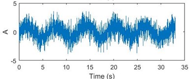
Fig. 1a) Sinusoidal signal; b) sinusoidal signal with -3 D white noise, c) 3D WVD plot, d) contour plot of WVD
a)
b)
c)
d)
Similarly, Fig. 2 shows the WVD plots for a discontinuous sinusoidal signal of the same frequency. The plot shows how the energy in the signal is discontinuous and unevenly distributed at that frequency.
Due to the windowing, there are non-zero values around the signal frequency component in both plots. The WVD plot is an excellent tool to detect the change in signal energy and henceforth, the fault that is causing it.
Fig. 2a) Discontinuous sinusoidal signal, b) discontinuous sinusoidal signal with –3 Db white noise, c) 3D WVD plot, d) contour plot of WVD
a)
b)
c)
d)
2.3. Modified Poincare mapping
The theory of chaos and nonlinear dynamics have spread across almost every field of contemporary science over the period of last ten decades. Chaotic method has provided new conceptual and theoretical methods to capture and understand the complex behaviours of nonlinear dynamic systems [20]. It is completely different from other methods used to analyse vibration signal.
In fluid mechanics chaos phenomena had been known, but only now chaotic vibrations have been observed in low-order mechanical systems. This has prompted the development of new ways of looking at dynamical solutions, such as Lyapunov exponents, fractal dimensions and Poincare Maps [20, 21]. Ehrich [1, 7], Myers et al., Abarbanel et al., Oppenheim et al., and Singer et al. were the first few to use chaotic vibration analysis to process signals [22-26].
By the principles of the Poincare Mapping, a time sequenced data of was recorded and by representing by , data point can be determined by the values of such that:
If a moving particle is displayed in the phase plane as, (, ), one can represent the motion discretely in a plot using and . This sequence of points forms a two-dimensional map of:
When the sampling times are chosen according to a specific position, this map is called a Poincare Map.
The primary importance of this study is to find a method to detect the location and severity of the bearing component failure in the rotor system. Hence, we are interested in every position of bearing and rotor running from 0° to 360°. This map is called the Poincare Map for a specific angle () position when the sampling rate is equal to the rotor speed. For a series of vibration data collected over cycles of revolutions, points of data in the Poincare Map are obtained.
The distance of each point to the origin, in a Poincare map can be calculated as shown in Eq. (7) and averaged as shown in Eq. (8):
The averaged points connected from 0° to 360° in polar coordinates gives us the average modified Poincare map [27-29] associated with the rotor speed. If the sampling rate is taken equal to the cage/ball carrier speed, then the modified Poincare map associated with the cage speed is obtained.
When the sampling rate is different and less than the rotor speed, multiple data points for each cycle of revolution are obtained. Let the rotor frequency to be , sampling frequency to be , the angle to be, , that the bearing rotates in the time between two data acquisition and is given by Eq. (9):
Plotting the vibration signal, with the angle, in polar coordinates gives the modified Poincare mapping.
3. Experimental setup
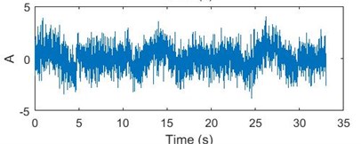
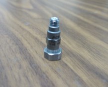
The test rig seen below in the Fig. 3 was fabricated to obtain the vibration signature of the bearing. The bearing used in the setup is SKF 6205-2Z. The speed of the motor is 1490 rpm (24.83 Hz). The motor is coupled to the shaft using a spider coupling. It is seen to it that there is no misalignment and unbalance in the rotor. To obtain the vibration signature of the bearings, accelerometers are placed on the bearing housing. An accelerometer of sensitivity, 101.3 mV/g, shown in Fig. 4, was placed on top of the test bearing housing to get the vertical vibration signature and an accelerometer of sensitivity 102.2 mV/g, shown in Fig. 5, was placed on the side of the same housing to get the horizontal vibration signature. These signals are collected through the controller Spider 81 and pre-processing and post processing is done on the signal using the Engineering Data Management (EDM) software interface. Six different bearings were studied using this experimental setup. The value for the bearing characteristic frequencies were calculated as, BPFI = 134.35 Hz, BPFO = 89.15 Hz, FTF = 9.93 Hz, BPF = 58.61 Hz, using the values, 9, 24.83 Hz, 0.312 mm, 1.535 mm and 0°.
Fig. 3Bearing test rig
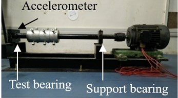
Fig. 4Accelerometer of sensitivity 101.3 mV/g
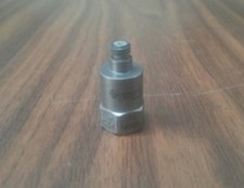
Fig. 5Accelerometer of sensitivity 102.2 mV/g
4. Identification of damaged bearings
The failures in a damaged bearing can be easily predicted by studying the trends in the vibration signature analysis methods mentioned in Section 2.
4.1. Failure prediction from FFT graphs
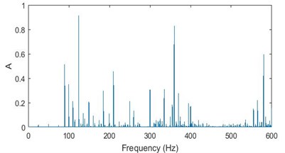
The FFT graphs can be only used to detect major defects in the bearing. The remaining faults are not detected by the FFT method. Hence, more powerful signal processing methods are therefore needed to unambiguously detect all faults.
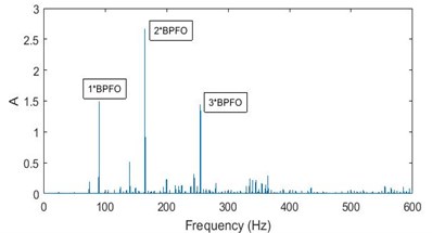
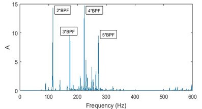
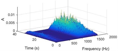
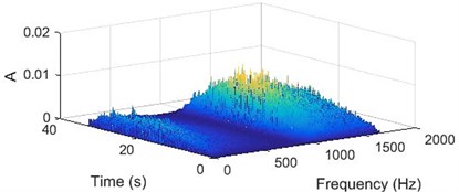
Fig. 6 show the FFT on the vibration signal acquired from good and two bad bearings [30-32]. From these figures it can be inferred that for a good bearing the amplitudes of the peaks in the FFT graph are small, as seen in Fig. 6(a), and for a bad bearing frequency corresponding to the failure and its harmonics are excited – the peaks seen in Fig. 6(b) are BPFO and its integral multiples and the peaks in Fig. 6(c) are BPF and its integral multiples [33]. The amplitude of vibration is measured and compared with vibration severity chart. If the amplitude reaches rough zone, preventive maintenance should be done. The artificial neural network and evolutionary algorithm are used to flag the user that the bearing needs to be changed [34, 35].
Fig. 6FFT graph for: a) a good bearing, b) a bearing with race failure, c) a bearing with ball failure
a)
b)
c)
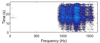
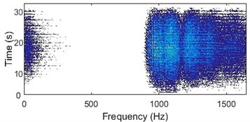
4.2. Failure prediction from WVD plots
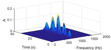
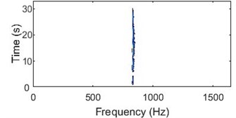
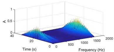
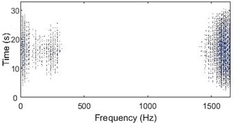
A signal acquired from a good bearing would consists mainly of vibration signature of the shaft rotation and the motor frequency. As the change in signal energy would be zero or negligible over the entire frequency spectrum, the WVD contour plot for such a signal would have vertical lines. Hence, it can be inferred that a bearing is in good condition if the WVD contour plot has vertical lines (lines parallel to time axis) as seen in Fig. 7(b).
Whereas, a signal acquired from a bad bearing would consists mainly of vibration signature of the bearing defect. As there would be continuous change in signal energy with a frequency corresponding to the failure, the WVD contour plot for such a signal would have horizontal lines (lines parallel to frequency axis), showing the discontinuity in the energy over the entire frequency spectrum. Fig. 8 shows the WVD plots for a bearing with a race failure and Fig. 9 shows the plots for a bearing with ball failure.
Fig. 7a) 3D plot and b) contour plot, of the WVD for a good bearing
a)
b)
Fig. 8a) 3D plot and b) contour plot, of the WVD for a bearing with race failure
a)
b)
Fig. 9a) 3D plot and b) contour plot, of the WVD for a bearing with ball failure
a)
b)
4.3. Failure prediction from modified Poincare mapping
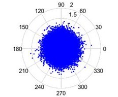
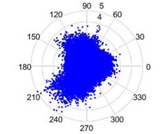
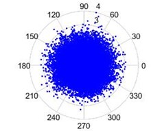
The modified Poincare Mapping is plotted as mentioned in Section 2.3, taking the vibration signature (displacement) as . Poincare mapping of vibration signature for a good bearing without defects, the plot will be concentric with the amplitude very less in comparison and few data points as outliers, as seen in Fig. 10(a). The bearing with a defect in the race, has the plot with skewed data points protruding in the direction the defect as seen in Fig. 10(b). The position of the protrusion gives us the location of the failure and the extent of protrusion gives us the severity of the failure. The modified Poincare map for bearing with defect in the ball is shown in Fig. 10(c). The amplitude is more in comparison to the plot of a good bearing and there are a lot of outliers at fixed angular intervals.
Fig. 10Modified Poincare mapping: a) a good bearing, b) a bearing with race failure, and c) a bearing with ball failure
a)
b)
c)
The data is acquired for three types of bearing (i) good bearing (ii) bearing with defect in race (iii) bearing ball failure. This data is acquired over a period, by running the setup shown in Fig. 3 and then these three methods are used for analysis to understand the type of failure.
The methods discussed in this section gives the notion of failed bearing based on the change in signature of FFT with respect to its amplitude and presence of side bands near different bearing failures. ANN and evolutionary algorithms are used to predict failure based of the amplitude reaching the severe zone of vibration severity chart. The presence of horizontal lines showing the discontinuity in the energy over the entire frequency spectrum in case of WVD vis-à-vis the discrete vertical lines in the contour plot of good bearing, gives a qualitative measure of bearing failure. In case of Poincare map, a polar plot of amplitude, the change in nature of plot, over a period, is taken and the observation of changes are corroborated with the maps of good bearing. The skewed nature of the graph in Fig. 10(b) with increased amplitude, gives a clear picture of bearing race failure in a direction. In case of Fig. 10(c), the amplitude increases in all directions and presence of outliers gives an indication of ball failure [6, 36].
5. Conclusions
Prediction of the condition of the bearing and the severity of the bearing failure using the vibration signature analysis methods like WVD and modified Poincare mapping is simple and efficient. In this paper, the prediction of bearing race failure and ball failure is studied experimentally and following broad conclusions are drawn.
1) FFT method of vibration signature analysis does not give us information about the time dependence of the vibration signal being analyzed. So, we need to take the signal periodically, analyses the signature and compare with standard signatures of failure as well as vibration severity chart.
2) WVD method of analysis also needs the periodic signature analysis and plot the WVD & contour plots. But the moment we see the horizontal lines in contour plot, we can see an eminent failure of the bearing and start comparing the signal amplitude with vibration severity chart. No expertise is needed to compare the FFT of signal with standards.
3) Poincare map method of analysis also needs the periodic signature analysis and plot the map. The advantage of this method is that we can easily find out the location of failure on the races of the bearing.
4) All these three methods have their uniqueness in some sense, but more exhaustive study is needed to conclude on superiority of any method.
5) It is proved that artificial neural network help in predicting exact time of failure. Combining these methods with artificial neural network will help in predicting exact time of failure.
References
-
Ehrich F. F. Some observations of chaotic vibration phenomena in high-speed rotor dynamics. Journal of Vibrations and Acoustics, Vol. 113, 1991, p. 50-57.
-
Rafiee J., Tse P. W. Use of autocorrelation in wavelet coefficients for fault diagnosis. Mechanical Systems and Signal Processing, Vol. 23, 2009, p. 1554-1572.
-
ASTM D6595-00, Standard Test Method for Determination of Wear Metals and Contaminants in Used Lubricating Oils or Used Hydraulic Fluids by Rotating Disc Electrode Atomic Emission Spectrometry, ASTM International, 05.03, 2011.
-
Nowicki A. N. Infrared Thermography Handbook. Volume 2, British Institute of Non-Destructive Testing, 2004.
-
Michael Robichaud J. Reference Standards for Vibration Monitoring and Analysis. Bretech Engineering Ltd, 2009.
-
Ruiwei Wu Identification of Bearing and Gear Tooth Damages from Experimental Vibration Signatures. M.S. Thesis, University of Akron, December 2007.
-
Ehrich F. F. Observations of subcritical super-harmonic and chaotic response in rotor dynamics. ASME Journal of Vibrations and Acoustics, Vol. 114, 1992, p. 93-100.
-
Myers C., Singer A., Shin F., Church E. Modeling chaotic systems with hidden Markov models. IEEE International Conference on Acoustics, Speech, and Signal Processing, 1992.
-
Myers C., Kay S., Richard M. Signal separation for nonlinear dynamical systems. IEEE International Conference on Acoustics, Speech, and Signal Processing, 1992.
-
Abarbanel H. D. I. Chaotic Signals and Physical Systems. IEEE International Conference on Acoustics, Speech, and Signal Processing, 1992.
-
Oppenheim A. V., Wornell G. W., Isabelle S. H., Cuomo K. M. Signal processing in the context of chaotic signals. IEEE International Conference on Acoustics, Speech, and Signal Processing, 1992.
-
Singer A. C., Wornel G. W., Oppenheim A. V. Codebook prediction: a nonlinear signal modeling paradigm. IEEE International Conference on Acoustics, Speech, and Signal Processing, 1992.
-
Choy F. K., Zhou J., Braun M. J., Wang L. Vibration monitoring and damage quantification of faulty ball bearing. ASME Journal of Lubrication Technology, Vol. 127, 2005, p. 776-783.
-
Robi Polikar The Wavelet Tutorial Part II. Fundamentals: The Fourier Transform and The Short Term Fourier Transform. http://users.rowan.edu/~polikar/WAVELETS/WTpart2.html.
-
RandallRobert Bond Vibration-based Condition Monitoring: Industrial, Aerospace and Automotive Applications. Willy Publishers, 2011.
-
Choy F. K., Jia Wei, Wu Ruiwei Identification of bearing and gear tooth damage in a transmission system. Tribology Transactions, Vol. 52, Issue 3, 2009, p. 303-309.
-
Flandrin P. Some features of time-frequency representations of multicomponent signals. Proceedings of International Conference on Acoustics, Speech, and Signal Processing, San Diego, USA, 1984.
-
Hlawatsch F. Interference terms in the Wigner distribution. Proceedings of the International Conference on Digital Signal Processing, Florence, Italy, 1984.
-
Velez Edgar F., Absher Richard G. Transient analysis of speech signals using the Wigner time-frequency representation. Proceedings of International Conference on Acoustics, Speech, and Signal Processing, Glasgow, Scotland, 1989.
-
Moon F. C. Chaotic Vibrations. John Wiley and Sons, Inc., 1987.
-
Farmer J. D., Ott E., Yorke J. A. The dimension of chaotic attractors. Physica D: Nonlinear Phenomena, Vol. 7, Issues 1-3, 1983, p. 153-180.
-
Myers C., Singer A., Shin F., Church E. Modeling chaotic systems with hidden Markov models. Proceedings of International Conference on Acoustics, Speech, and Signal Processing, San Francisco, USA, 1992.
-
Myers C., Kay S., Richard M. Signal separation for nonlinear dynamical systems. Proceedings of International Conference on Acoustics, Speech, and Signal Processing, San Francisco, USA, 1992.
-
Abarbanel H. D. I. Chaotic signals and physical systems. Proceedings of International Conference on Acoustics, Speech, and Signal Processing, San Francisco, USA, 1992.
-
Oppenheim A. V., Wornell G. W., Isabelle S. H., Cuomo K. M. Signal processing in the context of chaotic signals. Proceedings of International Conference on Acoustics, Speech, and Signal Processing, San Francisco, USA, 1992.
-
Singer A. C., Wornel G. W., Oppenheim A. V. Codebook prediction: a nonlinear signal modeling paradigm. Proceedings of International Conference on Acoustics, Speech, and Signal Processing, San Francisco, USA, 1992.
-
Choy F. K., Zhou J., Braun M. J., Wang L. Vibration monitoring and damage quantification of faulty ball bearings. ASME Journal of Tribology, Vol. 127, Issue 10, 2005, p. 776-783.
-
Choy F. K., Wang L., Zhou J., Braun M. J. On-line vibration monitoring of ball bearing damage using an experimental test rig. AIAA Journal of Propulsion and Power, Vol. 23, Issue 3, 2007, p. 629-636.
-
Choy F. K., Wu R., Konrad D., Labus E. Damage identification of ball bearings for transmission systems in household appliances. Tribology Transactions, Vol. 50, Issue 1, 2007, p. 74-81.
-
Wang W. Early detection of gear failure by vibration analysis - interpretation of time-frequency distribution using image processing techniques. Mechanical Systems and Signal Processing, Vol. 7, Issue 3, 1993, p. 205-215.
-
Mankar R. D., Gupta M. M. Vibration based condition monitoring by using Fast Fourier Transform A case on a turbine shaft. Proceedings of International Conference on Industrial Automation and Computing (ICIAC), Nagpur, India, 2014.
-
Mustafa Özgür Yayli On the axial vibration of carbon nanotubes with different boundary conditions. Micro and Nano Letters, Vol. 9, Issue 11, 2014, p. 807-811.
-
Rao J. S. Vibratory Condition Monitoring of Machines. Narosa Publishing House, 2000.
-
Nikilesh Krishnakumar, Vishal Jain, Pravin Singru M. Development of predictive model for vibro-acoustic condition monitoring of lathe. Journal of Vibroengineering, Vol. 17, Issue 1, 2015, p. 229-242.
-
Garg A., Vijayaraghavan V., Tai K., Pravin M. Singru, Vishal Jain, Nikilesh Krishnakumar Model development based on Evolutionary framework for condition monitoring of a lathe machine. Measurement, Vol. 95, 2015, p. 95-110.
-
Warwick Tucker Computing accurate Poincaré maps. Physica D, Vol. 171, 2002, p. 127-137.
Cited by
About this article

The authors acknowledge BITS-Pilani and Department of Science and Technology – FIST Program for providing funding for the experimental setup.
