Structural state inspection using dual-tree quaternion wavelet transform

1. Introduction

Structural state inspection based on response-only data has recently become a focused research topic, because it does not require a theoretical or numerical model of the measured structure and it is appropriate for structure motivated by unavailable or inaccessible excitation [1-3]. These two advantages are very important for engineering applications.

The key of the response-only method is how to extract feature index being sensitive to small state change. Among the used features, the transmissibility is known as a linear system concept only depended on the intrinsic characteristics of structure. It defines how vibration (both amplitude and phase) is transmitted between two testing points, and provides complete information with respect to the dynamic behavior of the structure. This had given rise to the development of structural state inspection by using transmissibility [4-9]. In fact, the measured vibration value is just the projectional component of the real vibration in sensor’s sensitive direction. Hence, the measured transmissibility will deviate from its theoretical value unless the installation orientations of two sensors coincides strictly. Concerning this issue, the QTJT was proposed in our previous work and proved to be unrelated to installation orientation of the sensors, which was advantageous in practical applications [10].

Essentially, the QTJT employed data fusion to avoid only the influence of inconsistent installation orientations of the sensors. More powerful analytical tool should be employed to deal with the measurement uncertainty caused by noise. For example, Yi et al. described the correlation of four-channel signals in quaternion domain, and proposed augmented quaternion singular spectrum analysis (AQSSA) based on convex-optimization [11]. Combined convex-optimization and permutation entropy, they also improved tensor-based singular spectrum algorithm (TSSA) to map the vibration signal into a high-dimensional space, which further revealed the dynamic behavior of the original signals [12]. Both two methods were used for fault diagnosis of rolling bearing and obtained good results. Chen et al. trained a four-layer ANN to complete fault diagnosis by using single channel transmissibility [13]. The ANN has strong ability of nonlinear mapping and fault tolerance. It can overcome the input noise to some extent. However, the initial weights of ANN usually need to be adjusted for many times to ensure the network convergence, which results in complicated and time-consuming calculation. And so far, there is no clear rule but an empirical formula to determine the best neural unit number of hidden layer of ANN.

Another way to overcome the measurement uncertainty is to increase the testing sample capacity and utilize the statistical information. For example, Mao and Todd quantified connection stiffness loss by using root-mean-square error directly calculated from the changes of measured transmissibility [14]. The more typical approach is multivariate statistical process monitoring (MSPM). The main idea of MSPM is to decompose the high dimensional training data into low dimensional latent space firstly, and then project the testing data to the latent space to get the monitoring statistic [15-17]. In most MSPM methods, the training data derive from multiple samples but the testing data derive from single sample. To overcome the measurement uncertainty of testing data, it is reasonable to construct testing data based on multiple samples also. Suppose multiple transmissibilities constitute a matrix, which is equivalent to an image in terms of data structure. In this case, structural state inspection converts to problem of image pattern recognition. The QWT was widely used in image pattern recognition due to its representation of quaternion magnitude-phase, which has characteristic of near shift-invariance and the ability to encode phase shifts [18-21].

Based on the above analysis, a state inspection method using dual-tree QWT combined with QTJT was described in this work. The feature image was constructed based on multiple QTJTs from the same state. The magnitude-phase derived from QWT coefficients of the feature image was considered as state feature index. And the difference of the state feature indexes was denoted by the Euclidean distance, which was also utilized as the state indicator. The availability of suggested method was demonstrated by an actual experiment.

2. Theoretical description

2.3. State inspection using QWT and QTJT

In this work, the modular vectors of multiple QTJTs from the same state were used to construct a state matrix. An equivalent grayscale feature image was obtained via simple scaling transformation of the elements in state matrix. In Fig. 1(a), each row of the image corresponded to a transposed modular vector of one measured QTJT from the same state. In Fig. 1(b), the measured QTJTs were from different states. It can be seen that different samples from the same state contained overall similarity but small local differences caused by measurement uncertainty, while the samples from different states showed obvious distinction.

Fig. 1The equivalent grayscale image composed of transposed modular vector of measured QTJTs

a) The QTJTs from the same state

b) The QTJTs from different states

Before state inspection, the state matrix $V_{si}^{m\times n}$ for each known state $i$ was constructed firstly, where $m$ was the length of QTJT and $n$ was the amount of QTJTs. Similarly, matrix $V_{tj}^{m\times n}$for unknown testing state $j$ was also constructed. Then the dual-tree QWT was employed to get the magnitude-phase matrix $A{F}_i$and $A{F}_j$. Theoretically, if $V_{si}^{m\times n}$ and $V_{tj}^{m\times n}$ belong to the same state, their corresponding magnitude-phase characteristic embedded in $A{F}_i$ and $A{F}_j$must be close to each other.

The first row of $AF$ indicates the low-frequency magnitude-phase characteristic of original image. The magnitude $\left|Q_{LL}\right|$ takes good low-pass characteristic in both the horizontal and vertical direction, and it is also the approximate representation of the original image in the next scale. Meanwhile, the phase (${\phi }_{LL},{\theta }_{LL},{\psi }_{LL}$) contains the local image shifts and image edge details. Compared with the magnitude-phase characteristic in specific direction, i.e., the last three rows in $AF$, the low-frequency magnitude-phase characteristic contains more complete information of original image. Furthermore, the data size of low-frequency magnitude-phase characteristic is only a quarter of $AF$, which is similar to the data dimension reduction in MSPM. So, the low-frequency magnitude-phase characteristic was selected as the state feature index in this work.

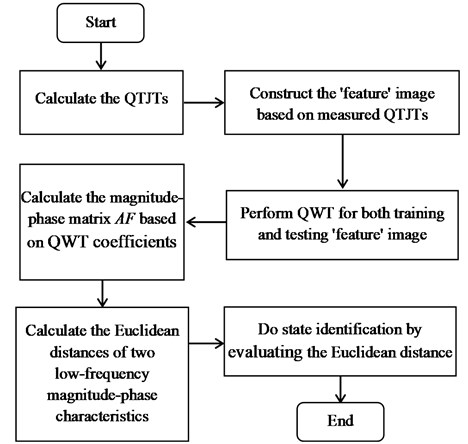
From the above, state inspection can be completed by evaluating the closeness of the state feature index between $A{F}_i$and $A{F}_j$. Specifically, testing state $j$ can be judged as known state $i$ when their Euclidean distance is the minimal. The flow chart of this method is summarized as Fig. 2. Since the calculation result for each step is uniquely determined, the whole process is clear and unidirectional with no detection or adjustment loop.

Fig. 2The flow chart of the QWT-based method

3. Experiment and discussion

Based on a real test platform of ballastless track, an experiment was performed. During the experiment, four fasteners between two testing points were loosed in turn. So, five structural states were achieved. The experimental process was just in keeping with that in Ref. [10] except for the motivation times being 40 instead of 20. The valid frequency was selected from 0.2 kHz to 1.7 kHz. Thus, the length of QTJT was 152 because the frequency resolution was 9.76 Hz. All the QTJTs from state 1 was illustrated in Fig. 3, together with the average QTJT from each state. In Fig. 3(a), the legend was not given because there was no enough space for the large amount of QTJTs. Actually, the line type was unified as solid and the color code was cycled every seven QTJTS. Again, the conclusion can be drawn that the QTJTs from the same state coincide approximatively, but the QTJTs from different states disaccord. The relative inconsistency in Fig. 3(a) mainly derived from the measurement uncertainty caused by instrument noise, environmental noise such as passing vehicles around the test platform, tiny changes of the exciting position, etc.

Here, four measured QTJTs from the same state were used to construct a feature image. So, a total of 10 feature images with size of 152×4 were obtained for each state. The former six images were considered as training images from known state and the last four images were used as testing ones from unknown state. Then state inspection was performed according to section 2.3. It was no doubt that higher level of quaternion wavelet decomposition meant higher frequency resolution. But it required more QTJTs to construct big feature image so as to increase calculation cost. Actually, QTJTs from the same state coincided approximatively, so the feature image had no rich textures. Therefore, high decomposition level was not necessary based on overall consideration. Here, the decomposition level was selected as 2. This resulted in $AF$ taking the same size with state matrix. And the size of low-frequency magnitude-phase characteristic was as same as one QTJT. The filter bank used in QWT was designed according to Ref. [25].

All the known feature images were ordered in sequence according to the state No. Thus, the testing feature image from state $i$ should correspond to known images $6\times \left(i-1\right)+1~6i$. The inspection result of QWT-based method was summarized in Table 1, where the first column showed the serial number of the matching image from known state, and the second column showed identification results.

Fig. 3The measured QTJT

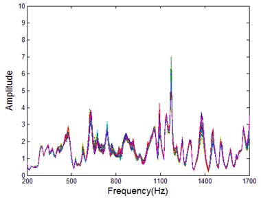
a) All QTJTs from state 1

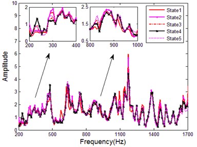
b) Average QTJT of each state

In order to test the performance of QWT-based state inspection method, it was compared with K-LT method which was expounded in our previous work [10]. Here, the former 30 QTJTs were training data and the latter 10 QTJTs were testing data. Likewise, all the training QTJTs were ordered in sequence. Thus, given a testing QTJT from state $i$, the serial number of its matching training QTJT should lie in $30\times \left(i-1\right)+1~30i$. The inspection result of K-LT method was summarized in Table 2.

According to Table 1 and Table 2, the QWT-based method got 100 % correct inspection rate, but the K-LT method got one misidentification in state 3. The effect of the two method looks a lot like, but different in deed. If the testing state is state $i$, in theory, any Euclidean distance lied in $6\times \left(i-1\right)+1~6i$ should be smaller than other ones when QWT-based method was used, and any Euclidean distance lied in $30\times \left(i-1\right)+1~30i$ should be smaller than other ones when K-LT method was used. The Euclidean distances of two arbitrary testing samples from state 3 using above two methods were illustrated in Fig. 4. It was seen that the QWT-based method got relative clear and regular result, but the K-LT method got not only one misidentification but also relative confused result even though the minimal Euclidean distance was correct matched. This indicated that the K-LT method might get relative higher chance of misidentification for weak damage.

Fig. 4The Euclidean distances of two arbitrary testing samples from state 2

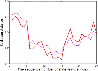
a) The QWT-based method

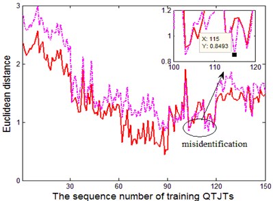
b) The K-LT method

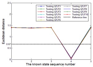
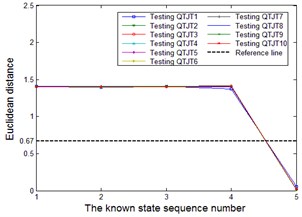
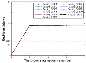
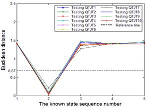
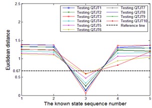
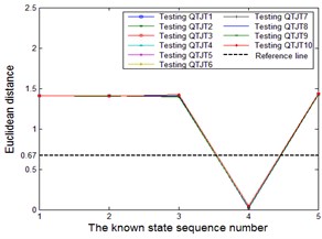
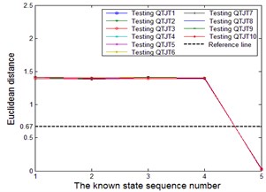
The QWT-based method was also compared with ANN method. Based on MATLAB, a three-layer BP ANN was created and trained. The normalized modular vector of the measured QTJT was utilized as the input, and the corresponding expected output was a $n$-dimensional vector, where $n$ was the amount of known state. If the input belonged to state $i$, the $i$th element of the expected output vector was 1 but others were 0. The learning rate of ANN was 0.05, the error threshold of objective function was 10^-3 and the maximum iterations were 1000. For each state, the former 20 measured QTJTs were utilized as training QTJTs, the latter 10 measured QTJTs were utilized as verification QTJTs to adjust the ANN structure, and the latest 10 measured QTJTs were utilized as testing QTJTs. For each testing QTJT, we calculated the Euclidean distances between its actual output vector and the expected output vectors of all the known state, and then judged the testing state was just one specific known state when their ANN outputs matched up to each other.

In this work, we premised the difference of corresponding elements of matching vectors should be no more than 0.3. So, the matching vectors must get the minimal Euclidean distance which was less than $\text{0.3}\sqrt{\text{5}}$ ≈ 0.67 at the same time due to five experimental states. Given a set of random initial values of the network weights, the ANN converged to the pre-set precision and got the structure of 152-12-5 after 12 iterations. The Euclidean distance results for all the five experimental states were illustrated in Fig. 5(a)-5(e).

Fig. 5The Euclidean distances between actual output of the testing QTJTs and the expected output vectors of all the known states. a)-e) testing QTJTs from state 1-5 with ANN structure of 152-12-5 f)-j) testing QTJTs from state 1-5 with ANN structure of 152-14-5

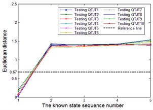
a)

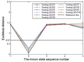
b)

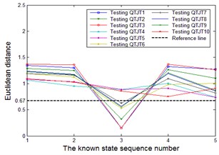
c)

d)

e)

f)

g)

h)

i)

j)

As shown in Fig. 5(c), the testing QTJT4, QTJT 5 and QTJT 10 of state 3 were misidentified. Moreover, the misidentifications of both ANN and K-LT method were focused on state 3 simultaneously.

As mentioned above, there is no clear rule but an empirical formula to determine the best neural unit number of hidden layer of ANN. Usually, the training accuracy of ANN can be improved by increasing the neural unit number of hidden layer, but in the meantime, the training efficiency may be reduced due to complex network structure. Here, the ANN was retrained with structure of 152-14-5. Given a set of new random initial values of the network weights, the ANN converged to the pre-set precision after 8 iterations, and then the state inspection was redone with the new ANN. The Euclidean distance results for all the five experimental states were illustrated in Fig. 5(f)-5(j). In this case, all the testing QTJTs were identified correctly, but the relatively worse Euclidean distance results were still obtained in state 3, as shown in Fig. 5(h). This indicated that the measured QTJTs from sate 3 were polluted more seriously than others. Note that the cutoff value was just a user-defined value by experience. Here the cutoff value less than 0.3 will lead to worse identification results according to Fig. 5(c) and Fig. 5(h).

Note that both two ANNs with different structure met the pre-set precision but got different inspection result in this work. Moreover, the ANN structure and the initial values of network weights affected the training efficiency. These were the issues that required attention when ANN method was employed. In a word, the QWT-based method got similar inspection effect but clearer and simpler computation process than ANN method, as well as better performance to overcome the measurement uncertainty than K-LT method.

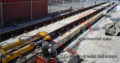
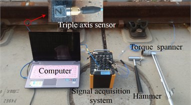
Luo et al. had proved that the longitudinal stress of the rail affected the vibration characteristics of the continuous welded rail track structure [26]. In order to verify this idea, a new experiment was performed by using a LG-900 hydraulic rail tensor to change the longitudinal stress of the rail, as shown in Fig. 6. Before the longitudinal stress changed, all the fasteners of the whole track structure were loosened. The hydraulic rail tensor was utilized to provide a new stress. Then torque spanners were used to re-lock all the fasteners so as to ensure the same locking force of the fasteners before and after longitudinal stress changes.

Fig. 6The experimental scene and equipment

a) The schematic diagram of experimental scene

b) The actual test platform of ballastless track

c) The used experimental equipment

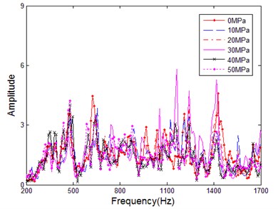
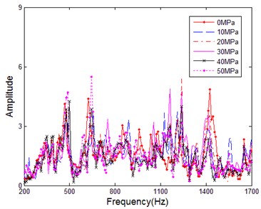
Given a specific longitudinal stress, the four fasteners between the same two testing points were also loosened one after another. Here, six tension stresses were provided, i.e., 0 MPa, 10 MPa, 20 MPa, 30 MPa, 40 MPa and 50 MPa. For each locking condition at one specific stress, 20 measured QTJTs were acquired. For each longitudinal stress, the average of all the 20 measured QTJTs belonged to the same locking condition was calculated. The average QTJT of the first two locking condition was illustrated in Fig. 7. It was seen that there were obvious differences among the average QTJT from the same lock condition but different longitudinal stress. Therefore, the structural state should be thought to have changed when the longitudinal stress changed to a certain degree even though any else condition remained the same. In this work, we considered that a total of 30 states were obtained. The state number was ordered following the rules in Table 3.

Fig. 7The average QTJT from different longitudinal stress

a) All fasteners fastened

b) One fastener loosened

Based on the new experimental data, state inspection using QWT-based method was performed firstly. A total of 5 feature images with size of 152×4 were obtained for each state. The former three images were considered as training images from known state and the latter two images were used as testing ones from unknown state. According to Table 3, all the known feature images were ordered in sequence. Thus, the testing images from state $i$ should correspond to known images $3\times \left(i-1\right)+1~3i$. The state inspection result was summarized in Table 4, in which 100 % correct identification rate was obtained again.

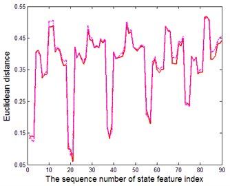
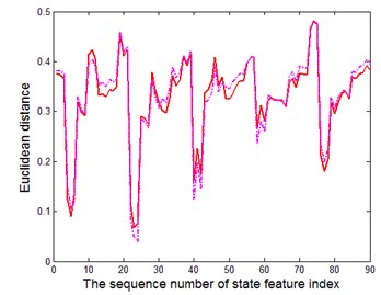
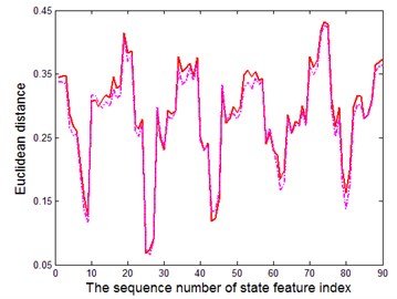
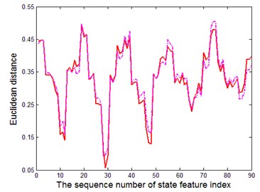
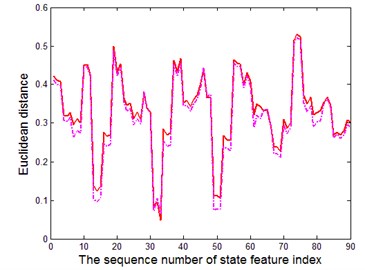
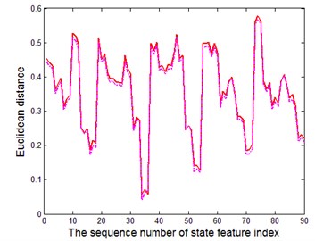
In order to present the inspection result more intuitively, the Euclidean distances of the two testing samples in locking condition 2 at each longitudinal stress were illustrated in Fig. 8.

Fig. 8The Euclidean distances of two testing samples in locking condition 2

a) At 0 MPa

b) At 10 MPa

c) At 20 MPa

d) At 30 MPa

e) At 40 MPa

f) At 50 MPa

The experimental result indicated that the resolution of QWT-based method for longitudinal stress change of the rail was superior to 10 MPa. According to the railway rail standards, the coefficient of linear expansion of the rail is $\alpha =$ 0.0118 mm/(m·℃), the elasticity modulus of the rail is $E=$ 2.1×10⁵MPa, and the cross-sectional area of the rail is 7.745×10^-3m². When the rail is completely locked, i.e., no longitudinal extension was permitted, the longitudinal force of the rail caused by temperature change of 1 ℃ can be given by:

The cross-sectional area of the oil cylinder of LG-900 hydraulic rail tensor was 3.352×10^-3 m². So, the longitudinal force corresponding to stress change of 10 MPa could be calculated as 10 MPa×3.352×10^-3m²= 33520 N. Thus, the equivalent resolution of QWT-based method for temperature change was superior to 33520 N /19192.11 N×1℃ = 1.75 ℃. For the reason of large experimental workload, smaller longitudinal stress change was not performed.

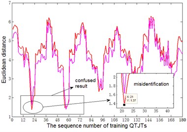
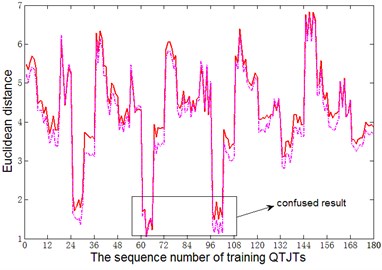
Subsequently, the new experimental data was also handled by K-LT method. This time, one misidentification still occurred in state 10, moreover, the obviously confused results were obtained in state 11. Part of inspection result of K-LT method was summarized in Fig. 9, where only six training QTJTs and two arbitrary testing QTJTs were illustrated in order to evaluate the regularity of the detection result compared with Fig. 4(a).

Frankly speaking, both the QWT-based method and K-LT method looked “ideal” in this work. The “ideal” classification result indicated that the QTJT was sensitive to full loose of one fastener in spite of the longitudinal stress, which could be considered as small change of the track structure. Actually, the ANN method was also employed at last. The three-layer BP ANN failed to converge to the pre-set precision after several attempts. In this work, no complex network structures were tried.

Fig. 9The Euclidean distances of two arbitrary testing samples using K-LT method

a) QTJTs from state 10

b) QTJTs from state 11

4. Conclusions

Learning from technology of image pattern recognition and MSPM, state inspection method using dual-tree QWT combined with QTJT was described. Multiple measured QTJTs were used to form a state feature image. Then the Euclidean distance between low-frequency magnitude-phase characteristics of different state feature images were utilized as the state indicator. The suggested method inspected the similarity of two feature images based on both magnitude and phase that contained the local image shifts and edge details. Moreover, it also reduced the influence of measurement uncertainty of single measured QTJT because it took overall consideration of multiple measured QTJTs. It was compared with K-LT and ANN method through a real experiment, and proved to be the integrated optimal method that got clearer and simpler computation process than ANN method, as well as better performance to overcome the measurement uncertainty than K-LT method. In addition, it was also proved that the longitudinal stress of object structure should be taken into consideration during state inspection based on vibration characteristic such as QTJT (transmissibility). For the suggested method, the resolution of the longitudinal force of rail was superior to10 MPa which is equivalent to temperature change of 1.75 ℃ for a completely locked railway structure.

This work still emphasized on the extraction of the state feature index and the definition of the state indicator instead of classification method. The suggested method only identified the presence of state changes. Therefore, further research should be done to develop it to identify the level and location of state changes. Compared to other method, it needed more measured QTJTs. Actually, this was not a real problem with modern technology of signal acquisition and storage.