Novel bearing fault diagnosis model integrated with dual-tree complex wavelet transform, permutation entropy and optimized FCM

Ma, Ping; Zhang, Hongli; Fan, Wenhui; Wang, Cong

doi:10.21595/jve.2017.18278

Journal of Vibroengineering

Browse Journal

Submit article

Published: 31 March 2018

Check for updates

Novel bearing fault diagnosis model integrated with dual-tree complex wavelet transform, permutation entropy and optimized FCM

Ping Ma¹

Hongli Zhang²

Wenhui Fan³

Cong Wang⁴

^{1, 2, 4}College of Electrical Engineering, Xinjiang University, Urumqi, China

³Department of Automation, Tsinghua University, Beijing, China

Corresponding Author:

Hongli Zhang

Cite the article Download PDF

Downloads 1559

CrossRef Citations 2

Abstract

In order to enhance the capability of feature extraction and fault classification of bearings, this study proposes a feature extraction approach based on dual-tree complex wavelet transform (DTCWT) and permutation entropy (PE), using the fuzzy c means clustering (FCM) to identify fault types. The vibration signal of bearings can be decomposed into several wavelet components with DTCWT which can describe the local characteristics of vibration signals accurately. And the PE of each wavelet component, which can describe the complexity of a time series, is calculated to be regarded as the fault features. Then forming the standard clustering centers by the FCM, we defined a standard using the Hamming approach degree to evaluate the classification results in the FCM. In order to verify the effectiveness of the proposed approach, compared with two other typical signal analysis methods: ensemble empirical mode decomposition (EEMD) and variational mode decomposition (VMD), through extracting fault features, it required to identify the fault types and severities under variable operating conditions. The experimental results demonstrate that the proposed approach has a better accuracy and performance to diagnose a bearing fault under different fault severities and variable operating conditions. The proposed approach is suitable for a fault diagnosis due to its good ability to the feature extraction and fault classification.

1. Introduction

Bearings are the key components in the mechanical structure, and the condition monitoring and fault diagnosis are critical to ensure the normal operation of machinery and equipment. The process of bearing fault diagnosis mainly consists of the fault feature extraction and fault classification [1, 2]. In case of a bearing failure, the frequency band energy of vibration signals will change. If frequency band signal characteristics can be extracted, the bearing fault classification can be carried out. Therefore, the effective extraction of fault feature is the key for a fault diagnosis.

The main problem of the feature extraction is how to process the different bearing vibration signals [3, 4]. Sometime-frequency analysis methods have been proposed to diagnose fault of rotating machinery in past few years, such as the empirical mode decomposition (EMD) [5, 6], local mean decomposition (LMD) [7], ensemble empirical mode decomposition (EEMD) [5, 8], and variational mode decomposition (VMD) [9]. The EMD is a self-adaptive method, for analyzing nonlinear and non-stationary signals to decompose the signals into a few intrinsic mode functions (IMFs). Each IMF is regarded as a mono-component [10]. Like with EMD, LMD decomposes the signals into a few product functions (PFs), each PF is a product of envelope and frequency modulated signals, from which the instantaneous frequency can be derived [11]. Yet the EMD has some drawbacks, including end effects, mode mixing and border effect problem. So, the EEMD has been proposed to eliminate the mode mixing problem of EMD [12]. The EMD, LMD and EEMD belong to recursive mode decomposition, by contrast, the VMD transforms the signal decomposition into non-recursive, variational modal decomposition model, and has better noise robustness [9, 13]. Thus, these time-frequency analysis methods, which combine the auto regressive model (AR), singular value decomposition (SVD) [2, 14], entropy-based method [8, 15, 16] and support vector machine (SVM) [9, 17], are widely used in the bearing fault diagnosis. However, there are some different problems in these methods. As mentioned above, the EMD and LMD also have mode combination and border effect problems, and they are all affected by the sampling frequency. The EEMD decomposition process is affected by the parameters so that it still has illusive components [12, 17]. Similarly, the VMD also is affected by the parameter determination [18].

So far, the discrete wavelet transforms (DWT) and second-generation wavelet transform (SGWT) have gained enormous applications for signal processing and bearing fault diagnosis in the literatures [19-21]. The DWT has the advantages of low entropy, multi resolution, flexible selection of substrates. While the main disadvantage of DWT consists in that it only decomposes the lowest frequency sub-band of signals and lacks the shift invariance, which may weaken the identification of fault features [22]. The SGWT is a wavelet transform based on a lifting scheme, but it also lacks the shift invariance and has severe aliasing in the process of decomposition. In order to overcome the defects of the above wavelet, the dual-tree complex wavelet transform (DTCWT) was initially proposed by Kingsbury [23], and Selesnick [24] who turned it up to the dyadic case. It was demonstrated that the performance of DTCWT was better than that of DWT and SGWT. The DTCWT retains the excellent properties of complex wavelet transform, and uses the dual-tree filter form to ensure the perfect signal reconstruction. Therefore, the dual tree complex wavelet transform is a kind of wavelet transform. It has good properties of approximate shift invariance, good directional selectivity, limited data redundancies, perfect reconstruction and high computational efficiency [24]. Because the DTCWT enjoys many attractive properties such as nearly shift-invariance and reduced aliasing which may be suitable to both the surveillance and diagnosis of rotating machine. And it has been used in the image processing [25], signal noise reduction processing [26] and engine fault diagnosis [27] etc.

In this literature, a new technique is proposed based on the DTCWT and permutation entropy (PE) to extract fault features in bearing vibration signals. The PE is an entropy-based method to analyze the signals complexity [28]. The permutation entropy is used in the statistical measuring method. It describes the local order structure and complexity of a time series via phase space reconstruction, and gets a great importance to the nonlinear behavior of the time series. It has been applied in many fields with the advantages of simplicity, robustness and invariance to nonlinear monotonous transformations [16, 29]. The wavelet components gained from the DTCWT can accurately describe the local characteristics of vibration signals, and the PEs of wavelet components can reflect more useful fault information. Therefore, in this study, the PE of a wavelet component is calculated to be regarded as the signal feature, and it represents the features of different signal types and is used to separates different faults. Meanwhile, the standard fuzzy C means clustering (FCM) is used to identify fault types, and the hamming approach degree is introduced to FCM to evaluate the result of clustering. the FCM is one of the most widely used algorithms in fuzzy clustering, which divides the samples of high similarity into the same category via iteration and optimization of the objective function [30]. And it also has been widely applied in the fault detection and diagnosis [31, 32].

The rest of this paper is organized as follows. The DTCWT, permutation entropy, optimized FCM are briefly reviewed in Section 2. Section 3 describes the proposed fault diagnosis method. Then in Section 4, the proposed approach is compared with the EEMD and VMD via extracting multiple fault signatures in the vibration signal and identifying the fault types and severities of bearings, using bearing vibration signals for validation. Finally, the conclusion is presented.

2. Related works

2.1. Dual-tree complex wavelet transform(DTCWT)

The DTCWT is a relatively recent enhancement to the DWT, which has important additional properties including nearly shift-invariant and directionally selective in two and higher dimensions [24]. The DTCWT uses two parallel DWTs (real tree and imaginary tree) with different low-pass and high-pass filters in each scale for signal decomposition and reconstruction. The decomposition and reconstruction of DTCWT are shown in Fig. 1.

Fig. 1DTCWT decomposition and reconstruction

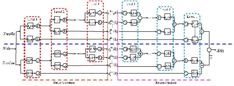
These two DWTs use two different sets of filters, and they satisfy the perfect decomposition and reconstruction. Let $ψ_{h} (t)$ and $ψ_{g} (t)$ represent the used two real-valued wavelets of DTCWT, and $φ_{h} (t)$ and $φ_{g} (t)$ are the corresponding scaling functions. A complex-valued wavelet $ψ (t)$ can be denoted as [26]:

1

ψ (t) = ψ_{h} (t) + i ψ_{g} (t) .

Then the DTCWT consists of two parallel wavelet transforms, therefore, according to the wavelet theory, the wavelet coefficients $d_{j}^{R e} (k)$ and the scaling coefficients $c_{J}^{R e} (k)$ of the above upper tree can be calculated by inner products as follows:

2

d_{j}^{R e} (k) = 2^{j / 2} \int_{- \infty}^{+ \infty} x (t) ψ_{h} (2^{j} t - k) d t, j = 1,2, \cdot \cdot \cdot, J,

3

c_{J}^{R e} (k) = 2^{J / 2} \int_{- \infty}^{+ \infty} x (t) φ_{h} (2^{J} t - k) d t,

where $j$ is the scale factor and $J$ is the maximum decomposition scale. Similarly, the wavelet coefficients $d_{j}^{I m} (k)$ and scaling coefficients $c_{J}^{I m} (k)$ of the above lower tree can be computed via Eqs. (4) and (5):

4

d_{j}^{I m} (k) = 2^{j / 2} \int_{- \infty}^{+ \infty} x (t) φ_{g} (2^{j} t - k) d t, j = 1,2, \cdot \cdot \cdot, J,

5

c_{J}^{I m} (k) = 2^{J / 2} \int_{- \infty}^{+ \infty} x (t) φ_{g} (2^{J} t - k) d t .

Then, the wavelet coefficients $d_{j}^{c} (k)$ and the scaling coefficients $c_{J}^{c} (k)$ of the DTCWT can be obtained by combining the dual tree output as follows:

6

d_{j}^{c} (k) = d_{j}^{R e} (k) + i d_{j}^{I m} (k), j = 1,2, \cdot \cdot \cdot, J,

7

c_{J}^{c} (k) = c_{J}^{R e} (k) + i c_{J}^{I m} (k) .

In the decomposition process, the input signal through the low-pass and high-pass filters, respectively. Since the signal frequency is divided into high-pass and low-pass, the bandwidth of the filtered output signal is only a half of the original signal. According to the sampling theorem of bandlimited signals, it is possible to reduce the sample rate by half without losing any information. Therefore, using binary sampling in the decomposition is reasonable, and the number of the obtained wavelet coefficients reduced by half with the depth of decomposition.

So, the complex wavelet coefficients and last-level scaling function coefficient are reconstructed to correspondingly obtain the detail signals at all levels and the approximation signal at the last level by the following equations:

8

d_{j} (t) = 2^{\frac{(j - 1)}{2}} [\sum_{n} d_{j}^{R e} (k) ψ_{h} (2^{j} t - n) + \sum_{m} d_{j}^{I m} (k) ψ_{g} (2^{j} t - m)], j = 1, \cdot \cdot \cdot, J,

9

c_{J} (t) = 2^{\frac{(J - 1)}{2}} [\sum_{m} c_{J}^{R e} (k) φ_{h} (2^{J} t - m) + \sum_{n} c_{J}^{I m} (k) φ_{g} (2^{J} t - n)],

where $m$ and $n$ are the lengths of the adopter filters.

Finally, the reconstructed signal $x' (t)$ is equal to the sum of all detail signals and approximation signal:

10

x^{'} (t) = c_{J} (t) + \sum_{j = 1}^{J} d_{j} (t) .

In the literature [24], it was proposed to design methods for dual-tree filters based on the half-sample delay condition. In this paper, (13, 19) – tap near symmetry biorthogonal filters are used at the first level, and the 14-tap linear phase filters produced by the Q-shift solution are used at the level except the first one. For more detailed information about the design of dual-tree filters in this paper, please refer to the literature [33].

2.2. Basic principle of permutation entropy

Permutation entropy (PE) is used to analyze the data complexity [28]. The permutation entropy is a statistical measuring method that has been effectively applied in many fields. The basic principle of PE is described as follows.

For a time series ${x (i), i = 1,2, \cdot \cdot \cdot, N}$ , a $d$ -dimensional delay embedding matrix is expressed as:

11

\begin{array}{l} X (1) = \{x (1), x (1 + τ), \cdot \cdot \cdot, x (1 + (d - 1) τ)\}, \\ X (2) = \{x (2), x (2 + τ), \cdot \cdot \cdot, x (2 + (d - 1) τ)\}, \\ X (i) = \{x (i), x (i + τ), \cdot \cdot \cdot, x (i + (d - 1) τ)\}, \\ ⋮ \\ X (N - (d - 1) τ) = \{x (N - (d - 1) τ) x (N - (d - 2) τ) \cdot \cdot \cdot x (N)\}, \end{array}

where $d$ denotes the number of the embedding dimension, $τ$ is the time delay. For $d =$ 2, there are two possible ordinal patterns of $X (i),$ namely $π_{1} = x (i) < x (i + τ)$ and $π_{2} = x (i + τ) < x (i)$ . The $d$ number of real values $X (i)$ can be arranged in an increasing order:

12

x (i + (j_{1} - 1) τ) \leq x (i + (j_{2} - 1) τ) \leq x (i + (j_{d} - 1) τ),

where $j$ represents the index in the column of embedding vector’s element and $1 \leq j_{i} \leq d$ . In general, there are just $d!$ possible order patterns.

If there are two or more elements having the same value, e.g. $x (i + (j_{1} - 1) τ) = x (i + (j_{2} - 1) τ)$ , we can sort the original positions for $j_{1} \leq j_{2}$ and $x (i + (j_{1} - 1) τ) \leq x (i + (j_{2} - 1) τ)$ can be recorded. Any $X (i)$ is uniquely mapped onto $π = (j_{1}, j_{2}, \cdot \cdot \cdot, j_{d})$ , which is one of the $d!$ permutations of $d$ distinct symbols. When each such permutation is considered as a symbol, then the reconstructed trajectory in the m-dimensional space is represented by a symbol sequence $S_{d}$ . We can say that $X (i)$ has a permutation $π$ , if and only if $π$ is unique in $S_{d}$ and satisfies Eq. (11).

For each permutation $π$ , the relative frequency can be calculated as follows:

13

p (π) = \frac{N u m b e r {X (i) h a s t y p e π | 1 \leq i \leq N - (d - 1) τ}}{N - (d - 1) τ} .

According to the Shannon’s entropy, the permutation entropy $H_{p} (d)$ of order $d$ for the time series is defined as:

14

H_{P} = - \sum_{π} p (π) \ln (p (π)) .

2.3. Optimized fuzzy $C$ means clustering

The FCM is the most classical clustering algorithm based on the objective function. Its central message is that each data point is associated with a cluster through a membership degree. And this technique divides a collection of data points into fuzzy groups and finds a cluster center in each group such that a cost function of a dissimilarity measure is minimized [31].

For a data sample $X = {x_{1}, x_{2}, \cdot \cdot \cdot, x_{N}}$ , giving the fuzzy membership matrix $U = [u_{i j}]_{c \times N}$ and the clustering center $C = [c_{1}, c_{2}, \cdot \cdot \cdot, c_{c}]^{T}$ , the most popular clustering method for identifying optimal fuzzy $c$ -partitions in $X$ is associated with the generalized least-squared errors functional [31]:

15

\begin{array}{l} \{\begin{array}{l} m i n {J (U, C^{T})} = \sum_{i = 1}^{N} \sum_{j = 1}^{c} u_{i j}^{m} d_{i j}^{2}, \\ s . t . \sum_{i = 1}^{c} u_{i j} = 1, \forall j = 1, \cdot \cdot \cdot, n, \end{array} \\ d_{i j}^{2} = {‖x_{j} - c_{i}‖}_{A}^{2} = (x_{j} - c_{i})^{T} A (x_{j} - c_{i}), \end{array}

where $m \in [1, + \infty)$ is weighting exponent, $N$ and $c$ represent the number of the data samples and clustering centers, respectively. $U$ is fuzzy $c$ -partitions in $X$ . $c_{i}$ is the center of cluster $i$ . The squared distance $d_{i j}^{2}$ between $x_{j}$ and $c_{i}$ is computed using metric matrix $A .$ $A$ is positive-definite ( $n \times n$ ) weight matrix. $\sum_{i = 1}^{N} \sum_{i = 1}^{c} (u_{i k})^{m} d_{i k}^{2}$ represents the overall weighted sum of generalized $A$ -errors due to replacing $X$ by $C$ .

Then, the extremum problem with constraint condition converts to the problem of unconstrained condition by introducing the operator $λ = [λ_{1}, \cdot \cdot \cdot, λ_{n}]$ :

16

\begin{array}{l} \bar{J} (U, C^{T}, λ) = J (U, c_{1}, \cdot \cdot \cdot, c_{c}) + \sum_{j = 1}^{N} λ_{j} (\sum_{i = 1}^{c} u_{i j} - 1) = \sum_{i = 1}^{c} \sum_{j = 1}^{N} u_{i j}^{m} d_{i j}^{2} + \sum_{j = 1}^{n} λ_{j} (\sum_{i = 1}^{c} u_{i j} - 1) . \end{array}

In the FCM algorithm, the fuzzy partitioning is obtained by an iterative optimization of the above function (16). The membership functions and cluster centers are updated by the following:

17

c_{i} = \frac{(\sum_{j = 1}^{N} u_{i j}^{m} x_{j})}{\sum_{j = 1}^{N} u_{i j}^{m}}, 1 \leq i \leq c,

18

u_{i j} = \frac{1}{\sum_{k = 1}^{c} {(\frac{d_{i j}}{d_{k j}})}^{2 / (m - 1)}}, 1 \leq j \leq N, 1 \leq k \leq c .

Conditions expressed in Eqs. (17) and (18) are necessary, but not sufficient. They provide means for optimizing $\bar{J}$ via simple Picard iteration, by looping back and forth from Eq. (17) to (18) until the iterate sequence shows but small changes in successive entries of $c_{i}$ or $u_{i j}$ .

The iteration can be stopped when the following iteration termination condition is satisfied:

19

m a x_{i j} \{|{u_{i j}}^{k + 1} - {u_{i j}}^{k}|\} < ε,

where $k$ is the iteration number and $ε$ is 0.00001 which satisfies a termination criterion.

The FCM algorithm consists of a series of iterations using Eqs. (17) and (18), which determine the cluster centers and membership matrix as follows:

Step 1). Definition of the number of cluster centers $c$ . The weighting exponent $m =$ 2. Choose an initial fuzzy membership matrix $U$ , and the number of iterations $k$ is 0.

Step 2). Calculation of the clustering center $C$ of all samples according to Eq. (17).

Step 3). Update of the fuzzy membership matrix $U$ by a new computed $u_{i j}$ using Eq. (18).

Step 4). Objective function calculation. If the difference between adjacent values of the objective function is less than the iteration termination criterion $ε$ then the iteration terminates. Otherwise, return to step 2.

In order to determine the classification accuracy of FCM, we propose an optimized FCM.

In this algorithm, we define a principle of hamming approach degree. Given the dataset $X = {x_{1}, x_{2}, \cdot \cdot \cdot, x_{N}}$ , $x \subset R^{m}$ , The $X$ contain samples of $c$ states, which has $c$ clustering centers. $C = [c_{1}, c_{2}, \cdot \cdot \cdot, c_{c}]^{T},$ $c \subset R^{m} .$ For a test dataset $T = {t_{1}, t_{2}, \cdot \cdot \cdot, t_{N}},$ $t \subset R^{m},$ define $N = [N_{1}, N_{i}, \cdot \cdot \cdot, N_{c}]$ to be a hamming approach degree. In order to determine whether the data sample $t_{i}$ belongs to the data sample category at the state $i$ for calculating hamming approach degree $N_{i}$ between the test sample $t_{i}$ and the clustering center $c_{i}$ under the state $i$ :

20

N_{i} = 1 - \frac{1}{m} \sum_{k = 1}^{m} |c_{i k} - t_{k}|, i = 1, \cdot \cdot \cdot, c .

For data sample $t_{i}$ , find the state that has the maximum hamming approach degree, and this data sample $t_{i}$ can be determined as it belongs to this state. In this paper, when the difference of the maximum hamming approach degree in 2 states is less than 0.01, that it cannot be identified or can be wrong.

3. Bearing fault diagnosis based on DTCWT-PE and optimized FCM

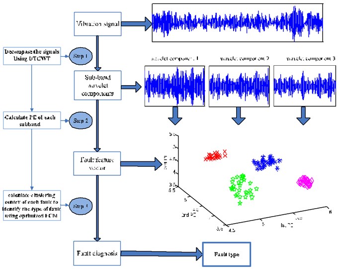
A method based on DTCWT, PE and optimized FCM is proposed for bearing fault diagnosis in this section. The procedure of this method is illustrated in Fig. 2 and summarized as follows:

Step 1) Perform the DTCWT for a vibration signal. In this step, each vibration signal is divided into 30 segments, and each segment contains 1024 points. According to the principle of DTCWT, each segment is decomposed into a few sub-band wavelet components. In this paper, the methods of EEMD and VMD are used for a comparison.

Step 2) For sub-band wavelet components of each segment, calculate the PE of three former wavelet sub-band components that contain more information, and it can be made up a 3×30 dimensional fault feature matrix. In this paper, DTCWT-PEs, EEMD-PEs, VMD-PEs are all calculated to make a comparison.

Step 3) Use the optimized FCM method to identify the type of fault. For vibration signals of different faults, it considers some part fault feature matrix obtained by step 2 as a data sample, using the FCM method, we calculate the clustering center of each data sample. And we regard the rest of fault feature matrix as a test data sample, calculating the hamming approach degree between cluster center of each fault to the test data. The fault is identified as a fault type when the test data and cluster center of this fault have the maximal Hamming approach degree.

Fig. 2Sketch of bearing fault diagnosis method

4. Experimental verification

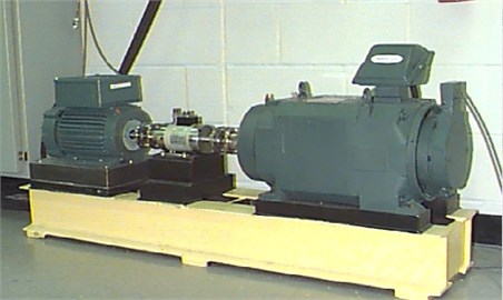
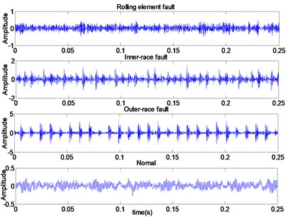
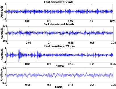
In this study, the bearing data are obtained from the Bearing Data Center of the Case Western Reserve University [34],to verify the effectiveness of the proposed method. And the data are obtained from a fault injection test of 6205-SKF deeply grooved ball bearings. The test rig consists of a 2-horse power motor, a torque transducer, a dynamometer, and control electronics (not shown), as shown in Fig. 3(a). Vibration data is collected using accelerometers, which are attached to the housing with magnetic bases. Accelerometers were placed at the 12 o’clock position at both the drive end and fan end of the motor housing. The test bearing supports the motor shaft and motor loads of 0 to 3 horsepower (hp) (corresponding to motor speed of 1797, 1772, 1750 and 1720 rpm). Single point faults were introduced to the inner race, rolling element and outer race of the test bearing using electro-discharge machining with fault diameters of 0.1778 millimeters, 0.3556 millimeters and 0.5334 millimeters. The sampling frequency is 12 kHz for drive end bearing experiments. Let’s take 1772 rpm as an example, the time domain waveforms of vibration signals under four working states are shown in Fig. 3(b). And Fig. 3(c) gives the vibration signals of rolling element fault with different fault diameters. Because of the non-stationary and nonlinear characteristics of the vibration signals, the DTCWT method is used to decompose them into a set of wavelet components.

Fig. 3a) Bearing test rig, b) vibration signals under four operating states, c) vibration signals of rolling element fault with different fault diameters

a) Bearing test rig, b) vibration signals under four operating states, c) vibration signals of rolling element fault with different fault diameters

a)

b)

c)

4.1. Feature extraction based on DTCWT and PE

In this section, each group of the vibration data is divided into several segments, and each segment contains 1024 points. Decompose each segment into a few wavelet components using the DTCWT. Then, calculate the PE of each signal component and regard it as the fault feature vectors.

In order to assess the advantages of the proposed approach, it is compared with several widely used feature extraction methods. In this paper, we choose DTCWT, EEMD and VMD to decompose signals into several components, and the PE groups can be calculated separately. The EEMD and VMD decompose signals into a few intrinsic mode functions (IMFs). Each IMF is regarded as a component. As the principles of DTCWT, EEMD and VMD are different, and the number of signal components is different for the same data, the number of the PEs is different similarly. But we know that there is the most dominant fault information from former mono-components, thus three former signal components can be considered and calculated. So, three PEs of each segment of vibration data can be regarded as the fault feature vectors.

Groups of feature vectors can be gained from each segment of vibration data. In this work, each vibration data is divided into 30 groups, and each group contains 1024 points. The detail of test dataset is shown in Table 1.

Table 1Detail of test dataset

	Health state	Fault width	Motor load (operating condition)
	Health state	Millimeters	0 hp	1 hp	2 hp	3 hp
1	Normal	–	90 grs	–	–	–
	Inner-race fault	0.1778	30 grs	30 grs	30 grs	30 grs
	Rolling element fault	0.1778	30 grs	30 grs	30 grs	30 grs
	outer-race fault	0.1778	30 grs	30 grs	30 grs	30 grs
2	Normal	–	90 grs	–	–	–
	Inner-race fault	0.3556	30 grs	30 grs	30 grs	30 grs
	Rolling element fault	0.3556	30 grs	30 grs	30 grs	30 grs
	outer-race fault	0.3556	30 grs	30 grs	30 grs	30 grs
3	Normal	-	90 grs	–	–	–
	Inner-race fault	0.5334	30 grs	30 grs	30 grs	30 grs
	Rolling element fault	0.5334	30 grs	30 grs	30 grs	30 grs
	outer-race fault	0.5334	30 grs	30 grs	30 grs	30 grs
4	Normal	–	30 grs
	Inner-race fault	0.1778, 0.3556, 0.5334 0.1778, 0.3556, 0.5334 0.1778, 0.3556, 0.5334		30, 30, 30 grs
	Rolling element fault			30, 30, 30 grs
	Outer-race fault			30, 30, 30 grs
grs: groups, hp: horsepower

4.1.1. Fault features extraction under variable operating conditions

The fault of bearings consists of inner-race fault, rolling element fault, and outer-race fault, the motor loads changes can be made under the variable operating conditions of bearings. As the motor loads influence the vibration intensity, then they influence the extracted PEs. It may lead to a mixture of features of different fault types. So, this is necessary to confirm the performance of diagnosis under variable operating conditions.

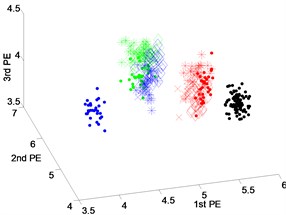
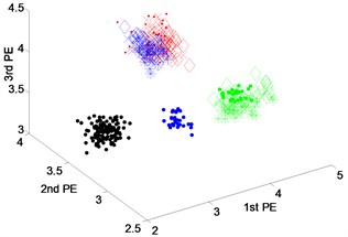
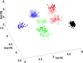
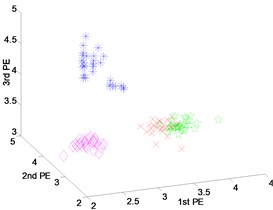
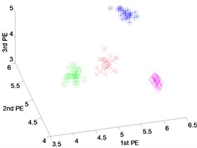
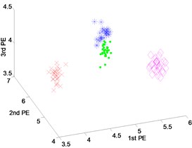
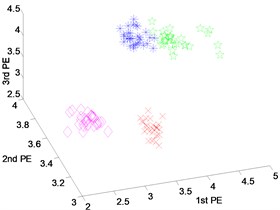
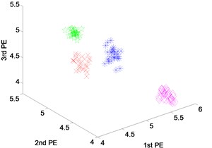
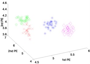
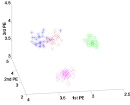
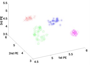
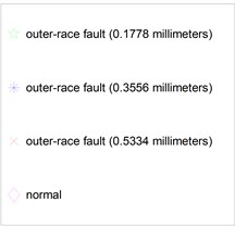
In this part, we consider the fault features extraction of different fault types under variable operating conditions (motor loads of 0 to 3 horsepower). Datasets 1-3 from table 1 are prepared for different fault severities under different operating conditions, and each dataset contains 13 subsets. For each segment of original signal, groups of three-dimensional fault features under different operating conditions are obtained by DTCWT-PEs, EEMD-PEs and VMD-PEs. Then scatter plots of DTCWT-PEs, EEMD-PEs and VMD-PEs for different fault severities under variable operating conditions are shown in Fig. 4-6.

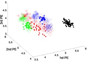
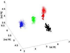
Fig. 4 shows the scatter plots of the fault feature extracted from dataset 1 using DTCWT-PEs, EEMD-PEs and VMD-PEs. Among the Fig. 4(a) and (b), the scatter plots of EEMD-PEs and VMD-PEs have the mixing phenomena. Features of three fault types at different operating conditions do not cluster very well, and there is a large overlap between three fault types clustering in EEMD-PEs. From the scatter plots of DTCWT-PEs in Fig. 4(c), we can see that features of different fault types at four operating conditions cluster well and are far away from the health state. So, three fault types and normal states can be separated effectively.

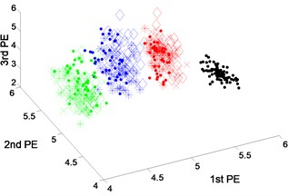
The scatter plots of feature vectors are obtained from dataset 2 using DTCWT-PEs, EEMD-PEs and VMD-PEs, as shown in Fig. 5. In Fig. 5(b), where the features between rolling element fault and inner-race fault obtained by VMD-PEs occur with the mixing phenomena. In Fig. 5(a) and (c), the scatter plots of the feature vectors obtained from EEMD-PEs and DTCWT-PEs are gathered well at variable operating conditions, and the separation between the fault types is clear.

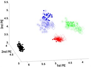
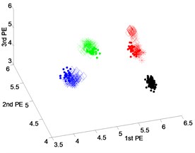
Fig. 6 presents the scatter plots of feature vectors gained from dataset 3 with fault diameters equal to 0.3556 millimeters by three techniques. From Fig. 6(a), it can be seen that the fault features between rolling element fault and outer-race fault using EEMD-PEs have an overlap. And there are some mixing phenomena of feature vectors between inner-race fault and outer-race fault of VMD-PEs in Fig. 6(b). From Fig. 6(c), we can see that the features extracted by DTCWT-PEs are obviously separable.

According to the analysis of Fig. 4-6, comparing the fault features extraction results using EEMD-PEs and VMD-PEs, we can see that the fault features extraction results of DTCWT-PEs have a great advantage. The feature vectors of different fault types at four operating conditions cluster well. At the stage of three different fault severities, different fault types and normal states are effectively separated. It indicates that the proposed fault feature extraction method of DTCWT-PEs has better performance at variable operating conditions.

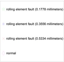
Fig. 4Scatter plot of: a) EEMD-PEs, b) VMD-PEs and, c) DTCWT-PEs for fault feature extraction results of dataset 1 under variable operating conditions

a) EEMD-PEs

b) VMD-PEs

c) DTCWT-PEs

d)

Fig. 5Scatter plot of: a) EEMD-PEs, b) VMD-Pes and, c) DTCWT-Pes for fault feature extraction results of dataset 2 under variable operating conditions

a) EEMD-PEs

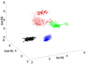
b) VMD-PEs

c) DTCWT-PEs

d)

Fig. 6Scatter plot of: a) EEMD-PEs, b) VMD-PEs and, c) DTCWT-Pes for fault feature extraction results of dataset 3 under variable operating conditions

a) EEMD-PEs

b) VMD-PEs

c) DTCWT-PEs

d)

4.1.2. Fault feature extraction for different fault severities

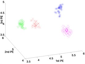
In order to demonstrate the feature extraction performance of DTCWT-PEs in identifying different fault severities, vibration data is analyzed at different fault severities. The detail of the extracted feature dataset with different fault severities is shown in Table 1 (dataset 4). The analyzed vibration data containing the normal state and three-faults state with fault diameters of 0.1778 millimeters, 0.3556 millimeters and 0.5334 millimeters, and we select the vibration data at the motor loads of 1 horsepower as an example. The features of normal state, inner-race fault state, rolling element fault state and outer-race fault state are extracted respectively by DTCWT-PEs, EEMD-PEs and VMD-PEs. The scatter plots of the fault features at different fault severities are shown respectively in Fig. 7-9.

Fig. 7 shows the scatter plots of the fault features extracted from the rolling element fault with different fault severities and normal state using DTCWT-PEs, EEMD-PEs and VMD-PEs where the scatter plots of the feature vectors obtained from EEMD-PEs and DTCWT-PEs are gathered well and are far away from each other. In particular, the features vectors of Fig. 7(c) are more compact, and the separation of the different states is very clear. By contrast, in Fig. 7(b), the scatter plots of VMD-PEs have some mixing between the fault severities with 0.1778 millimeters and 0.5334 millimeters.

The scatter plots of feature vectors are obtained from the inner-race fault with different fault severities and normal state, as shown in Fig. 8. In Fig. 8(a) and (b), where the features obtained by EEMD-PEs and VMD-PEs of inner-race fault between the fault severities with 0.1778 millimeters and 0.5334 millimeters, the mixing phenomena occur. From the scatter plots of DTCWT-PEs in Fig. 8(c), we can see that the features of different fault severities cluster well and are far away from the health state, three fault severities and normal states can be separated effectively.

Fig. 9 shows the scatter plots of feature vectors gained from the outer-race fault with different fault severities and normal state by three techniques. From Fig. 9(a) and (b), it can be seen that the features of four states do not cluster very well, the features extracted by EEMD-PEs and VMD-PEs are mixed for different fault severities, especially in Fig. 9(b). The scatter plots of DTCWT-PEs are shown in Fig. 9(c). We can see that the feature vectors cluster well, and there is no mixing phenomena happened.

From the above analysis, we can determine that the feature are extracted from different fault severities by the EEMD-PEs and VMD-PEs occurred with mixing phenomena. While the features extracted from the DTCWT-PEs also have the capacity to be distinguished as different fault severities of three fault types, the features of different fault severities cluster well and are far away from each other. Therefore, the features extraction performance of DTCWT-PEs is better than that of EEMD-PEs and VMD-PEs for different fault severities.

Fig. 7Scatter plot of: a) EEMD-PEs, b) VMD-PEs and, c) DTCWT-PEs for fault feature extraction results with rolling element fault of dataset 4

a) EEMD-PEs

b) VMD-PEs

c) DTCWT-PEs

d)

Fig. 8Scatter plot of: a) EEMD-PEs, b) VMD-Pes and, c) DTCWT-PEs for fault feature extraction results with inner-race fault of dataset 4

a) EEMD-PEs

b) VMD-PEs

c) DTCWT-PEs

d)

Fig. 9Scatter plot of: a) EEMD-PEs, b) VMD-PEs and, c) DTCWT-Pes for fault feature extraction with outer-race fault results of dataset 4

a) EEMD-PEs

b) VMD-PEs

c) DTCWT-PEs

d)

4.2. Fault diagnosis by optimized FCM

In order to verify the performance of DTCWT-PEs in the fault identification, the optimized FCM is introduced to calculate the classification accuracy. In this step, we consider the diagnosis of all kinds of data under the same loads. Meanwhile, we use the fault data under known load conditions to identify the fault types of other load conditions. The detailed information of the data sample is shown in Table 2.

Table 2Detail of dataset

	Health state	Fault width	Motor load (working condition)
	Health state	Millimeters	0 hp	1 hp	2 hp	3 hp
1	Normal	–	40 grs	–	–	–
	Inner-race fault	0.1778	40 grs	40 grs	40 grs	40 grs
	Rolling element fault	0.1778	40 grs	40 grs	40 grs	40 grs
	Outer-race fault	0.1778	40 grs	40 grs	40 grs	40 grs
grs: groups, hp: horsepower

4.2.1. Fault diagnosis under same load

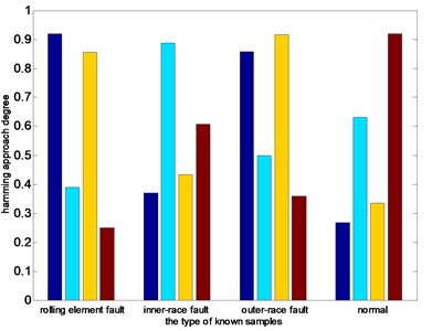
Under the motor load of 1 hp, 40 groups of data sample are extracted in turn from the normal, inner-race fault, outer-race fault and rolling element fault. Among them, the former 20 groups of four states are regarded as the known samples, using the FCM to get the standard cluster center separately, the last 20 groups of data are regarded as test samples, through the hamming approach degree calculation used to identify the fault types. The experimental results show that the fault recognition rates of extracted features using three techniques are 100 %. In order to further prove the effectiveness of the proposed method, the hamming approach degree between test samples and four known different states is calculated.

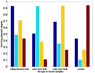
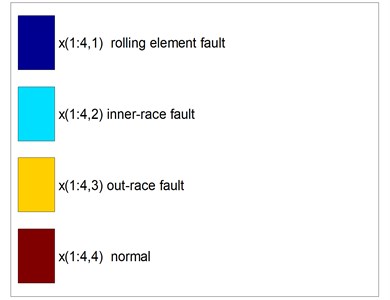
Fig. 10 shows the columnar distribution of the hamming approach degree between test samples and four different known states. From Fig. 10(a) and (b), we can see that the hamming approach degrees between test samples and corresponding state based on the EEMD-PEs and VMD-PEs are smaller than that ones based on the DTCWT-PEs. in addition, it can be seen in Fig. 10(b) that the maximum hamming approach degree is obviously close to the second largest hamming approach degree. In Fig. 10(c), when the type of test sample is the rolling element fault, inner-race fault, outer-race fault and normal, the maximum hamming approach degree between test samples and corresponding state is close to 1, that is obviously higher than the second largest hamming approach degree. The accurate recognition and clustering abilities of DTCWT-PEs are demonstrated. Therefore, the method of DTCWT-PEs can more accurately extract the characteristics of each state, the clustering effect is better, and it is easier to classify the faults automatically.

Fig. 10Distribution of average nearness

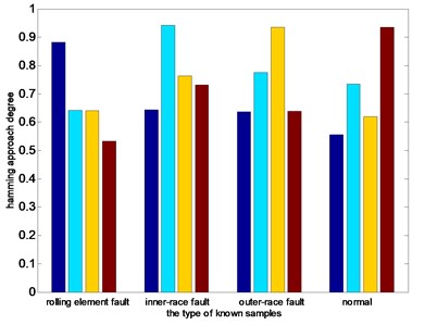
a) EEMD-PEs

b) VMD-PEs

c) DTCWT-PEs

d)

4.2.2. Fault diagnosis under variable load

Due to that the equipment safety is relatively high in engineering applications, the small probability of failures leads to the shortage of fault samples. The fault samples can only be collected under a certain condition sometimes. Therefore, it is significant to identify the fault types under different operating conditions by using the existing fault data under this specific condition. In this paper, the fault diagnosis of other three load conditions is carried out with the help of the clustering center of existing and known fault data under load 0. Test samples are taken from the load 1, load 2 and load 3, and each of them has 40 groups, and uses the hamming approach degree between test samples and existing known fault data to identify the fault type of a test sample. The classification results show that the proposed approach can achieve a good classification effect under all loads, and the fault recognition rate is still 100 %, e.g. the fault diagnosis results of test samples under load 2 by using the clustering center of existing known fault data under load 0 are listed, as shown in Table 3. Due to the fault signal changed under different loads, in EEMD-PEs, there are 2 outer-race fault data which are mistakenly diagnosed as an inner-race fault, and 3 inner-race fault data are diagnosed as a rolling element fault in the VMD-PEs. And we can see that the DTCWT usage can be effectively identified as the four-states type under load 1 with the help of the clustering center of existing fault data under load 0.

Table 3Fault diagnosis for load 2 by EEMD-PEs, VMD-PEs and DTCWT-PEs

		Normal	Inner-race fault	Outer-race fault	Rolling element fault
EEMD-PEs	Normal	40	0	0	0
	Inner-race fault	0	40	0	0
	Outer-race fault	0	2	38	0
	Rolling element fault	0	0	0	40
VMD-PEs	Normal	40	0	0	0
	Inner-race fault	0	37	0	3
	Outer-race fault	0	0	40	0
	Rolling element fault	0	0	0	40
DTCWT-PEs	Normal	40	0	0	0
	Inner-race fault	0	40	0	0
	Outer-race fault	0	0	40	0
	Rolling element fault	0	0	0	40

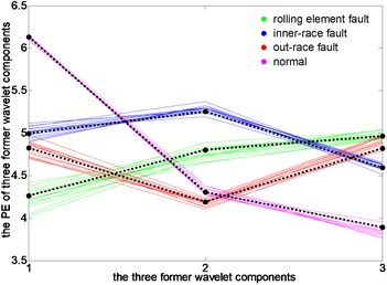
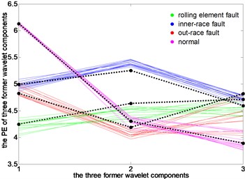
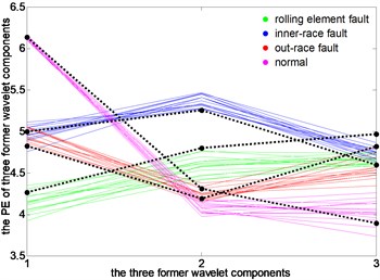
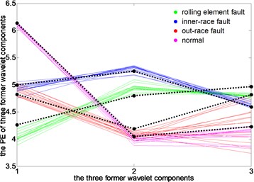
In this section, for a vibration signal under different loads, the PEs of three signal components decomposed from DTCWT-PEs are linked together, that forms the characteristic line of the test sample. Then the change trend of the characteristic line is analyzed under different loads relative to the characteristic line of the original cluster center obtained under the load of 0 hp, as shown in Fig. 11.

Fig. 11Run chart of original cluster centers and characteristics line of test samples

a) 0 hp load

b) 1 hp load

c) 2 hp load

d) 3 hp load

It can be seen that, under load 0, the characteristic lines of four states closely follow the black characteristic lines of a standard clustering center, thus the accuracy of clustering center extraction is proved. Under load 2, the characteristic line of rolling element fault is deviated from the clustering center firstly, and the characteristic line of normal state has some deviations. Under 1 hp load and 3 hp load, the characteristic lines of 4 states have a varying degree of deviation. Among them, the degree of characteristic lines of outer-race fault deviated from the clustering center is the biggest, and the normal state is the second one. Overall, when the motor load changes, the characteristic lines of a test sample under different operating conditions are all around the characteristic lines of clustering center under 0 hp load, which makes the fault recognition rate of rolling bearings be maintained at 100 %.

5. Conclusions

In this work, an approach for bearing fault identification is proposed based on the DTCWT, PE and optimized FCM. The basic idea is that the vibration signal is decomposed into several wavelet components by the DTCWT, calculating the PE of former three wavelet components. This approach regards them as the fault feature vectors, and then the algorithm of optimized FCM is introduced into the identified fault type. The experimental results verified that a more accurate classification had been obtained using DTCWT-PEs compared with EEMD-PEs and VMD-PEs. It was demonstrated that the proposed method had better ability to identify different faults types and different fault severities under different operating conditions.

It is shown that the proposed approach can accurately identify different fault severities, and has a good performance to resist variable operating conditions. Practically, the proposed feature extraction approach based on the DTCWT and PE in this paper is suitable for diagnosing a bearing fault due to that it has a strong performance of clustering and recognition. But the efficiency of this approach may be affected when the operating condition has some big changes. Therefore, a further research will mainly focus on improving the fault diagnosis capability under variable operating conditions.

References

Liu W. Y., Han J. G., Jiang J. L. A novel ball bearing fault diagnosis approach based on auto term window method. Measurement, Vol. 46, Issue 10, 2013, p. 4032-4037.

Publisher
Tian Y., Ma J., Lu C., et al. Rolling bearing fault diagnosis under variable conditions using LMD-SVD and extreme learning machine. Mechanism and Machine Theory, Vol. 90, 2015, p. 175-186.

Publisher
Liu H., Han M. A fault diagnosis method based on local mean decomposition and multi-scale entropy for roller bearings. Mechanism and Machine Theory, Vol. 75, 2014, p. 67-78.

Publisher
Lei Y., Lin J., He Z., et al. Application of an improved kurtogram method for fault diagnosis of rolling element bearings. Mechanical Systems and Signal Processing, Vol. 25, Issue 5, 2011, p. 1738-1749.

Publisher
Lei Y., Lin J., He Z., et al. A review on empirical mode decomposition in fault diagnosis of rotating machinery. Mechanical Systems and Signal Processing, Vol. 35, Issue 1, 2013, p. 108-126.

Publisher
Bin G. F., Gao J. J., Li X. J., et al. Early fault diagnosis of rotating machinery based on wavelet packets-empirical mode decomposition feature extraction and neural network. Mechanical Systems and Signal Processing, Vol. 27, 2012, p. 696-711.

Publisher
Cheng J., Yang Y., Yang Y. A rotating machinery fault diagnosis method based on local mean decomposition. Digital Signal Processing, Vol. 22, Issue 2, 2012, p. 356-366.

Publisher
Tabrizi A., Garibaldi L., Fasana A., et al. Early damage detection of roller bearings using wavelet packet decomposition, ensemble empirical mode decomposition and support vector machine. Meccanica, Vol. 50, Issue 3, 2015, p. 865-874.

Publisher
Dragomiretskiy K., Zosso D. Variational mode decomposition. IEEE Transactions on Signal Processing, Vol. 62, Issue 3, 2014, p. 531-544.

Publisher
Huang N. E., Shen Z., Long S. R., et al. The empirical mode decomposition and the Hilbert spectrum for nonlinear and non-stationary time series analysis. Proceedings of the Royal Society of London A: Mathematical, Physical and Engineering Sciences. The Royal Society, Vol. 454, Issue 1971, 1998, p. 903-995.

Publisher
Smith J. S. The local mean decomposition and its application to EEG perception data. Journal of the Royal Society Interface, Vol. 2, Issue 5, 2005, p. 443-454.

Publisher
Wu Z., Huang N. E. Ensemble empirical mode decomposition: a noise-assisted data analysis method. Advances in Adaptive Data Analysis, Vol. 1, 2009, p. 1-41.

Publisher
Ma Z. Q., Li Y. C., Liu Z., et al. Rolling bearings fault feature extraction based on variational mode decomposition and Teager energy operator. Journal of Vibration and Shock, Vol. 35, Issue 13, 2016, p. 134-139.

Search CrossRef
Cheng J., Yu D., Tang J., et al. Application of SVM and SVD technique based on EMD to the fault diagnosis of the rotating machinery. Shock and Vibration, Vol. 16, Issue 1, 2009, p. 89-98.

Publisher
Zhang S. Q., Sun G. X., Li L., et al. Study on mechanical fault diagnosis method based on LMD approximate entropy and fuzzy C-means clustering. Chinese Journal of Scientific Instrument, Vol. 34, Issue 3, 2013, p. 714-720.

Search CrossRef
Zhang X., Liang Y., Zhou J. A novel bearing fault diagnosis model integrated permutation entropy, ensemble empirical mode decomposition and optimized SVM. Measurement, Vol. 69, 2015, p. 164-179.

Publisher
Yang Y., Cheng J., Zhang K. An ensemble local means decomposition method and its application to local rub-impact fault diagnosis of the rotor systems. Measurement, Vol. 45, Issue 3, 2012, p. 561-570.

Publisher
Tang G. J., Wang X. L. Parameter optimized variational mode decomposition method with application to incipient fault diagnosis of rolling bearing. Journal of Xi’an Jiaotong University, Vol. 49, Issue 5, 2015, p. 73-81.

Search CrossRef
Yan R., Gao R. X., Chen X. Wavelets for fault diagnosis of rotary machines: a review with applications. Signal Processing, Vol. 96, 2014, p. 1-15.

Publisher
Djebala A., Ouelaa N., Hamzaoui N. Detection of rolling bearing defects using discrete wavelet analysis. Meccanica, Vol. 43, Issue 3, 2008, p. 339-348.

Publisher
Li Z., He Z., Zi Y., et al. Rotating machinery fault diagnosis using signal-adapted lifting scheme. Mechanical Systems and Signal Processing, Vol. 22, Issue 3, 2008, p. 542-556.

Publisher
Selesnick I. W. The design of approximate Hilbert transform pairs of wavelet bases. IEEE Transactions on Signal Processing, Vol. 50, Issue 5, 2002, p. 1144-1152.

Publisher
Kingsbury N. G. The dual-tree complex wavelet transform: a new technique for shift invariance and directional filters. IEEE Digital Signal Processing Workshop, Bryce Canyon, Vol. 86, 1998, p. 120-131.

Search CrossRef
Selesnick I. W., Baraniuk R. G., Kingsbury N. C. The dual-tree complex wavelet transform. IEEE Signal Processing Magazine, Vol. 22, Issue 6, 2005, p. 123-151.

Publisher
Lo E. H. S., Pickering M. R., Frater M. R., et al. Image segmentation from scale and rotation invariant texture features from the double dyadic dual-tree complex wavelet transform. Image and Vision Computing, Vol. 29, Issue 1, 2011, p. 15-28.

Publisher
Wang Y., He Z., Zi Y. Enhancement of signal denoising and multiple fault signatures detecting in rotating machinery using dual-tree complex wavelet transform. Mechanical Systems and Signal Processing, Vol. 24, Issue 1, 2010, p. 119-137.

Publisher
Wang F. T., Chen S. H., Yan D. W., et al. Noise reduction based on dual tree complex wavelet transform unfolding and its application in fault diagnosis. Journal of Mechanical Engineering, Vol. 50, Issue 21, 2014, p. 159-163.

Publisher
Bandt C., Pompe B. Permutation entropy: a natural complexity measure for time series. Physical Review Letters, Vol. 88, Issue 17, 2002, p. 174102.

Publisher
Zanin M., Zunino L., Rosso O. A., et al. Permutation entropy and its main biomedical and econophysics applications: a review. Entropy, Vol. 14, Issue 8, 2012, p. 1553-1577.

Publisher
Bezdek J. C. Pattern Recognition with Fuzzy Objective Function Algorithms. Springer Science and Business Media, 2013.

Search CrossRef
Gou M. F., Xu L. L., Liao X. R., et al. A vibration signal feature extraction method for distribution switches based on singular value decomposition of time-frequency matrix. Proceedings of the CSEE, Vol. 34, Issue 28, 2014, p. 4990-4997.

Search CrossRef
Jahromi A. T., Er M. J., Li X., et al. Sequential fuzzy clustering based dynamic fuzzy neural network for fault diagnosis and prognosis. Neurocomputing, Vol. 196, 2016, p. 31-41.

Publisher
Kingsbury N. Complex wavelets for shift invariant analysis and filtering of signals. Applied and Computational Harmonic Analysis, Vol. 10, Issue 3, 2001, p. 234-253.

Publisher
http://www.eecs.case.edu/laboratory/bearing.

Search CrossRef

Cited by

Experimental and theoretical investigation of CVT rubber belt vibrations

Adam Kot | Waldemar Łatas

(2021)

Preload state detection for precision spindle bearings based on multi-level classification

Xiaohu Li | Yanfei Zhang | Yuechen Han | Jun Hong

(2020)

About this article

Received

23 February 2017

Accepted

29 July 2017

Published

31 March 2018

SUBJECTS

Fault diagnosis based on vibration signal analysis

DOI

https://doi.org/10.21595/jve.2017.18278

Keywords

bearing fault diagnosis

features extraction

dual-tree complex wavelet transform

permutation entropy

optimized FCM

Acknowledgements

This work is supported by the National Science Foundation of China (Nos. 51767022, 51575469) and the outstanding Doctor Graduate Student Innovation Project (No. XJUBSCX-2016017).

This is an open access article distributed under the Creative Commons Attribution License, which permits unrestricted use, distribution, and reproduction in any medium, provided the original work is properly cited.

Previous article in issue Previous Next article in issue Next

Research article

2024 01 21

Rolling bearing fault diagnosis based on variational mode decomposition and weighted multidimensional feature entropy fusion

Na Lei, Feihu Huang, Chunhui Li

Research article

2023 09 08

Research on fault diagnosis method of bearing based on parameter optimization VMD and improved DBN

Yingqian Sun, Zhenzhen Jin

Research article

2019 11 15

Novel complete ensemble EMD with adaptive noise-based hybrid filtering for rolling bearing fault diagnosis

Xiaojun Song, Hongwei Sun, Liwei Zhan

Research article

2019 09 30

Bearing fault diagnosis based on feature extraction of empirical wavelet transform (EWT) and fuzzy logic system (FLS) under variable operating conditions

Fawzi Gougam, Chemseddine Rahmoune, Djamel Benazzouz, Boualem Merainani

P. Ma, H. Zhang, W. Fan, and C. Wang, “Novel bearing fault diagnosis model integrated with dual-tree complex wavelet transform, permutation entropy and optimized FCM,” Journal of Vibroengineering, Vol. 20, No. 2, pp. 891–908, Mar. 2018, https://doi.org/10.21595/jve.2017.18278

Copy Extrica

Copied to clipboard!

TY  - JOUR
DO  - 10.21595/jve.2017.18278
UR  - https://doi.org/10.21595/jve.2017.18278
TI  - Novel bearing fault diagnosis model integrated with dual-tree complex wavelet transform, permutation entropy and optimized FCM
T2  - Journal of Vibroengineering
AU  - Zhang, Hongli
AU  - Ma, Ping
AU  - Fan, Wenhui
AU  - Wang, Cong
PY  - 2018
DA  - 2018/03/31
PB  - JVE International Ltd.
SP  - 891-908
IS  - 2
VL  - 20
SN  - 1392-8716
ER  - 

Copy Ris

Copied to clipboard!

@article{Zhang_2018,
	doi = {10.21595/jve.2017.18278},
	url = {https://doi.org/10.21595/jve.2017.18278},
	year = 2018,
	month = {mar},
	publisher = {{JVE} International Ltd.},
	volume = {20},
	number = {2},
	pages = {891--908},
	author = {Hongli Zhang and Ping Ma and Wenhui Fan and Cong Wang},
	title = {Novel bearing fault diagnosis model integrated with dual-tree complex wavelet transform, permutation entropy and optimized {FCM}},
	journal = {Journal of Vibroengineering}
}

Copy Bibtex

Copied to clipboard!

[1]H. Zhang, P. Ma, W. Fan, and C. Wang, “Novel bearing fault diagnosis model integrated with dual-tree complex wavelet transform, permutation entropy and optimized FCM,” Journal of Vibroengineering, vol. 20, no. 2, pp. 891–908, Mar. 2018, doi: 10.21595/jve.2017.18278.

Copy IEEE

Copied to clipboard!

Zhang, Hongli, Ping Ma, Wenhui Fan, and Cong Wang. “Novel Bearing Fault Diagnosis Model Integrated with Dual-Tree Complex Wavelet Transform, Permutation Entropy and Optimized FCM.” Journal of Vibroengineering 20, no. 2 (March 31, 2018): 891–908. https://doi.org/10.21595/jve.2017.18278.

Copy Chicago

Copied to clipboard!

Novel bearing fault diagnosis model integrated with dual-tree complex wavelet transform, permutation entropy and optimized FCM

Abstract

1. Introduction

2. Related works

2.1. Dual-tree complex wavelet transform(DTCWT)

2.2. Basic principle of permutation entropy

2.3. Optimized fuzzy C means clustering

3. Bearing fault diagnosis based on DTCWT-PE and optimized FCM

4. Experimental verification

4.1. Feature extraction based on DTCWT and PE

4.1.1. Fault features extraction under variable operating conditions

4.1.2. Fault feature extraction for different fault severities

4.2. Fault diagnosis by optimized FCM

4.2.1. Fault diagnosis under same load

4.2.2. Fault diagnosis under variable load

5. Conclusions

References

Cited by

About this article

Related Articles

2.3. Optimized fuzzy $C$ means clustering