Automatic semantic segmentation and classification of remote sensing data for agriculture

Jadhav, Jagannath K.; Singh, R. P.

doi:10.21595/mme.2018.19840

Mathematical Models in Engineering

Browse Journal

Submit article

Published: 30 June 2018

Check for updates

Automatic semantic segmentation and classification of remote sensing data for agriculture

Jagannath K. Jadhav¹

R. P. Singh²

¹VTU University, Belagavi, Karnataka, India

²SSSUTMS, Madhya Pradesh, India

Corresponding Author:

Jagannath K. Jadhav

Cite the article Download PDF

Downloads 2851

CrossRef Citations 18

Abstract

Automatic semantic segmentation has expected increasing interest for researchers in recent years on multispectral remote sensing (RS) system. The agriculture supports 58 % of the population, in which 51 % of geographical area is under cultivation. Furthermore, the RS in agriculture can be used for identification, area estimation and monitoring, crop detection, soil mapping, crop yield modelling and production modelling etc. The RS images are high resolution images which can be used for agricultural and land cover classifications. Due to its high dimensional feature space, the conventional feature extraction techniques represent a progress of issues when handling huge size information e.g., computational cost, processing capacity and storage load. In order to overcome the existing drawback, we propose an automatic semantic segmentation without losing the significant data. In this paper, we use SOMs for segmentation purpose. Moreover, we proposed the particle swarm optimization technique (PSO) algorithm for finding cluster boundaries directly from the SOMs. On the other hand, we propose the deep residual network to achieve faster training process. Deep Residual Networks have been proved to be a very successful model on RS image classification. The main aim of this work is to achieve the overall accuracy greater than 85 % (OA > 85 %). So, we use a convolutional neural network (CNN), which outperforms better classification of certain crop types and yielding the target accuracies more than 85 % for all major crops. Furthermore, the proposed methods achieve good segmentation and classification accuracy than existing methods. The simulation results are further presented to show the performance of the proposed method applied to synthetic and real-world datasets.

1. Introduction

During the past few years, remote sensing (RS) on image processing is used for many real time applications. It is widely used to detect and classify the objects from land and under oceans, but now it is mainly used for the agricultural purpose such as crop mapping, forest inventory, land cover, crop mapping etc. [1]. The most widely used satellite for agriculture is LANDSAT 8. It contains operational land imager (OLI) and thermal infrared sensor (TIRS). It covers the landmass, agriculture and remote areas [2].

The RS images acquired by the OLI and the TIRS based LANDSAT satellite, measure the reflected and emitted energy from 11 bands, ranging from deep blue and violet (BAND 1) to long-wave infrared (band 11). The OLI with 8 band and the agriculture multispectral scenes mainly utilize the 6, 5, 2 bands. RS images are generally used for watching the urban extension and land cover changes at a medium to enable the advancement of urbanization [3].

The growth of the crop, crop types and land cover are classified based on the desired classifier technique [4]. Some of the classifiers used for classifications are, Support Vector Machine (SVM), Neural Network (NN), and Random forest (RF) etc. [5]. The SVM classifier is used for accurate segmentation without any losses. Moreover, it is very efficient for a land cover classification with overall accuracy (OA) is 75 %. But it consumes too-many resources and possesses large classification problems [6]. Then the neural network achieves OA of 74 %. It is mainly used for single data classification, so it cannot be used in multispectral images. After that, the RF-based classifier achieves OA of < 85 %. Moreover, this classifier is not efficient for multispectral data scenes.

Therefore, the deep learning-based classification method is used to achieve better classification accuracy [7]. The deep learning is a powerful technique in machine learning methodology to solve a wide range of task in image processing, remote sensing and computer vision [8]. In last few years, more studies used the DL (deep learning) approach for processing the RS imagery. DL have been proved to be an efficient method for hyper spectral, multispectral imagery and radar images in different land cover, crop type and other agricultural methods [9].

In terms of deep learning process, neural network is classified as supervised neural network and unsupervised neural network [10]. The unsupervised neural network is used for the image segmentation and missed data restoration. The supervised classification requires the learning information about the study region for training the detection module [11]. The unsupervised change detection procedures are applied on the multispectral images, that are acquired from sensors. These methods are mainly divided into preprocessing, semantic segmentation, and post processing [12]. The unsupervised CD strategies are also used for multispectral images, that detect the changes without earlier data and with a decreased computational weight [13]. The vast majority of them permit only the detection of quality of changes but do not separate various types of changes. This process reduces the critical loss of data, and improve the overall accuracy [14, 15].

Su T. [16] proposed an efficient paddy field mapping method by means of object-based image analysis and the bi-temporal data set, which is developed by Landsat-8 operational land imager. The proposed technique is tested using bi-temporal data set, which is acquired from landsat-8 over the Baoying Xian and the mapping accuracy. The efficiency of the proposed full form (SETH) algorithm is increased due to the red-black tree structure. The fully unsupervised selection method is combined with the image segmentation. Moreover, the object-based RF classifiers are tested to produce the accurate field classification. Normally, a good classification accuracy can be achieved by using bi-temporal data set. But, the classification and the segmentation are complicated for multispectral data scenes.

Maggiori E., et al. [17] presented a convolutional neural network for large scale remote sensing based image classifications. Despite their outstanding learning capability, the lack of accurate training data might limit the applicability of CNN models in realistic remote-sensing contexts. Consequently, they proposed a two-step training approach, that combines the use of large amounts of raw OSM data and a small sample of manually labeled reference. This was achieved by analyzing the role played by every layer in the network. Moreover, the multi-scale modules increase the level of detail of the classification without making the number of parameters explode, attenuating the tradeoff between detection and localization. The learning process is complicated for multiple object classes and non-pansharpened imagery.

Bargoti S. [18] projected an image segmentation for fruit detection and yield estimation. General purpose feature learning algorithms were utilized for image segmentation, followed by detection and counting of individual fruits. The image segmentation was performed using MS-MLP and a CNN. Within these architectures, they incorporated metadata to explicitly capture relationships between meta-parameters and the object classes. The metadata yielded a boost in performance with the MS-MLP network. Therefore, the improved segmentation performance with the CNN can also be translated in to more accurate crop detection using both detection algorithms. The architecture of the training and testing is not clearly given, as it needs better capabilities.

McCool C., et al. [19] presented the lightweight deep convolutional neural networks based on agricultural robotics. The key approach for training these models is to “distill” the knowledge from a complex pre-trained model considered to be an expert for the task at hand. Using this approach, they considerably improved their accuracy of robotic weed segmentation from 85.9 %, using a traditional approach, to 93.9 % using an adapted DCNN with 25M parameters able to process 155 regions per second. The downside to this highly accurate model is not able to be deployed for real-time processing on a robotic system. The FCN consists of a complicated DCNN such as VGG or GoogLeNet.

Pei W., et al. [20] introduced the object-based image analysis which was used to map the land use in the coal mining area. The mapping and detection of the land use change in the coal area using the object-based analysis. The Landsat images can be used to accurately extract the land use information’s in the coal mining area. It provides the fundamental information’s for the land use classifications in the mining areas. Therefore, the multi-temporal classifications results show the better accuracy and kappa coefficients than existing techniques. These observed trends in land use change could be a useful basis for ensuring compliance with environmental regulations or permitting in mining regions.

Ma L., et al. [21] offered object-based image analysis. The availability and accessibility of high resolution RS data create a challenge in RS image classification. To deal with these uncertainties and some limitations, the supervised classifications are used. Then the Meta-analysis technique provided a unique change to integrate the RS images. It provides a scientific guidance for RS research. The main objective of the system was to conduct a meta-analysis of results in existing studies. The extractor was given to dropout, which was successfully a way to increase the accuracy with a probability of 50 %. Thus, the saliency detection was a useful and efficient way to extract the patches from VHR images; And by the unsupervised learning method such as sparse auto encoder extract a high quality features from VHR and accuracy was greater or equal to SIFT-based technique. And by using SVM classifier the robust and efficiency can be learned. Thus, the unsupervised learning was an efficient approach for RS image classifications.

These literature works provide significant classification and feature determination for various data analysis. But, these methods lack some important significant parameters, such as accurate accuracy assessment, correct feature extraction and classifications. It cannot predict correct change detection results. Moreover, those work provides high error rates according to such parameters.

The main objective of the paper is to develop an automatic semantic segmentation and classifications for agriculture data. The proposed method initially gets the sufficiency and presentation in light of the close-by time of an image. The main aim of the proposed system is to evaluate the segmentation quality by finding the missed data and increase the crop mapping and land cover classification. The SOMs is used for segmentation of RS images and for finding missed values. The PSO optimized SOMs is introduced for reducing the optimization problem during segmentation. After segmentation, neural network model will be applied to classification task. Deep Residual Networks have been proven to be a very successful model on RS image classification. So, we use a CNN which outperforms better classification of certain crop types and yielding the target accuracies more than 85 % for all major crops. Finally, the proposed feature extraction technique is compared with the popular existing feature extraction techniques for detecting the changes.

Significant contribution of the paper with its advantages:

1) Modelling of an automatic segmentation and classification of the RS data for agriculture.

2) Representation of particle swarm optimization technique (PSO) algorithm for finding cluster boundaries of images directly from the SOMs.

3) The deep residual network achieves faster training process during classification.

4) The ResNet 101 Convolutional Neural Network (CNN) model is used for better classification of certain crop types.

5) The proposed work achieves good segmentation and classification accuracy greater than 85 % (OA > 85 %) as compared to existing methods.

6) Simulation and prediction of the proposed work is compared with several existing methods.

The rest of the manuscript is arranged as follows. Section 2mproposed work with the automatic semantic segmentation technique is used to segment the images in the multi-spectral image. Then the result analysis and the performance evaluation of the remote sensing data for the proposed method is discussed in Section 3. The overall conclusion for the automatic semantic segmentation is given in the last section.

2. Proposed methodology

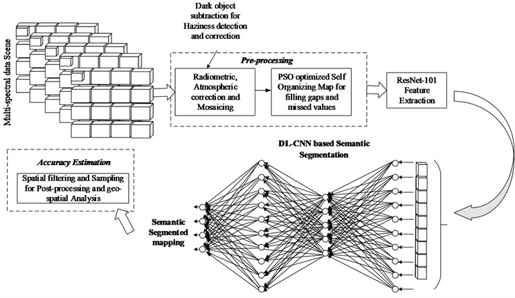
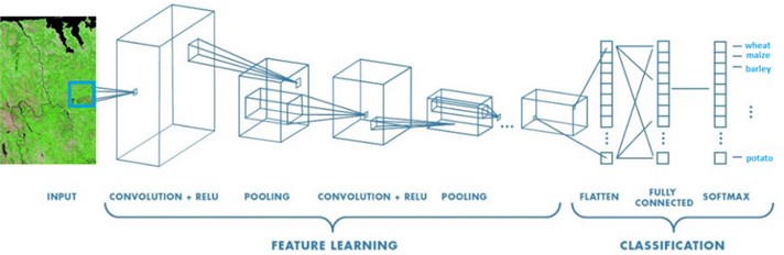
First, a RS multispectral agriculture scene is taken as our input data base. The proposed work is mainly divided into three modules: (i) pre-processing, (ii) semantic segmentation, (iii) post-processing (quality assessment). The architecture of the proposed work is given in Fig. 1.

2.1. Input database

The multispectral RS images are considered as a database for the proposed framework. In this paper, images are taken from the database and given as an input to the proposed automatic semantic segmentation technique:

1

Q_{i} = \sum f (x, y),

where $x$ , $y$ is a row and column value and $Q_{i}$ is a raw data.

2.2. Pre-processing

The pre-processing steps such as radiometric calibration, atmospheric correction, and mosaicking are performed on the image to obtain the detailed information about the remote sensing images.

Fig. 1Architecture of the proposed system

2.2.1. Radiometric calibration

Radiometric correction method is used to avoid the radiometric errors, while the geometric correction is to remove geometric distortion. Also, various atmospheric effects cause absorption and scattering of the solar radiation [22]. The key objective of radiometric correction is to recover the true radiance or the reflectance of the target. It is mainly used to improve the visual appearance of the image [23]. The radiometric correction is applicable by obtaining some of the steps given below.

Step 1: Conversion of digital number to spectral radiance.

During the execution of Level-1 product, the image pixels were converted into units of the absolute radiance by means of 32-bit floating point calculations. Then the pixel values are multiplied by using 100 and then converted to 16-bit integer which is prior to media output, maintain two digits of the decimal precision. The lower and the upper limit of the original rescaling factor is taken for the conversion of $Q_{c a l}$ back to the sensor spectral radiance. The following general equation is used to convert Digital Numbers (DNs) to radiance ( $L$ ):

2a

L_{λ} = (\frac{L M A X_{λ} - L M I N_{λ}}{Q_{c a l m a x} - Q_{c a l m i n}}) (Q_{c a l} - Q_{c a l m i n}) + L M I N_{λ},

or:

2b

L_{λ} = G_{r e s c a l e} \times Q_{c a l} + B_{r e s c a l e},

where:

3

G_{r e s c a l e} = \frac{L M A X_{λ} - L M I N_{λ}}{Q_{c a l m a x} - Q_{c a l m i n}},

4

B_{r e s a c l e} = L M I N_{λ} - (\frac{L M A X_{λ} - L M I N_{λ}}{Q_{c a l m a x} - Q_{c a l m i n}}) Q_{c a l m i n},

where $L_{λ}$ is spectral radiance at the sensors aperture [W/ (m² sr µm)], $Q_{c a l}$ is quantized calibrated pixel value [DN], $Q_{c a l m i n}$ is minimum quantized calibrated pixel value corresponding to $L M I N_{λ}$ [DN], $Q_{c a l m a x}$ is maximum quantized calibrated pixel value corresponding to $L M A X_{λ}$ [DN], $L M I N_{λ}$ is spectral at-sensor radiance that is scaled to $Q_{c a l m i n}$ [W/ (m² sr µm)], $L M A X_{λ}$ is spectral at sensor radiance that is scaled to $Q_{c a l m a x}$ [W/ (m² sr µm)], $G_{r e s c a l e}$ is band specific rescaling gain factor [W/ (m² sr µm)] [DN], $B_{r e s a c l e}$ is band specific rescaling bias factor [W/ (m² sr µm)].

The maximum quantized calibrated pixel value of 8 bit DN range is 0 to 255.

Step 2: Conversion of spectral radiance to atmospheric reflectance (TOA).

Conversion to TOA radiance. The product is delivered in 16bit unsigned integer format and rescaled to the top of atmosphere. The OLI and the TIRS bands data are converted to TOA spectral radiance by means of radiance rescaling factors provided on the metadata file:

5

L_{λ} = M_{L} Q_{c a l} + A_{L},

where, $L_{λ}$ is TOA spectral radiance (watts/ (m²·srad·µm)), $M_{L}$ is band specific multiplicative rescaling factor from the metadata file (Radiance multi-band $x$ , where $x$ is the band number), $A_{L}$ is band specific additive factor from the metadata, $Q_{c a l}$ is quantized and calibrated standard product pixel values (DN).

Conversion to TOA reflectance. The OLI spectral band data can be converted to the TOA reflectance by means of reflectance rescaling coefficients. The following equations are used to convert the DN values to the TOA reflectance for the operational land imager:

6

ρ λ = M_{ρ} Q_{c a l} + A_{ρ},

where $ρ λ$ is TOA planetary reflectance without correction for solar angle, $M_{ρ}$ is band-specific multiplicative rescaling factor from the metadata, $A_{ρ}$ is band-specific additive rescaling factor from the metadata, $Q_{c a l}$ is quantized and calibrated standard product pixel values (DN).

TOA reflectance with the correction for the sun angle is given as:

7

ρ λ = \frac{ρ λ'}{c o s (θ_{s z})} = \frac{ρ λ'}{s i n (θ_{S E})},

where $ρ λ$ is TOA planetary reflectance, $θ_{S E}$ is local sun evaluation angle. The scene center sun elevation angle in degrees is provided in the metadata (SUN_ELEVATION), $θ_{S Z}$ is local solar zenith angle; $θ_{S Z} = 90 ° - θ_{S E}$ . Therefore, for more exact reflectance value calculations, per pixel value of solar angles can be used as a substitute of the scene center solar angle, but the per pixel zenith angles are not simultaneously provided with the LANDSAT 8 yields.

2.2.2. Atmospheric correction

The atmospheric correction is mainly used to retrieving surface reflectance from the RS imagery. It is mainly used for removing effects of atmosphere on reflectance value in the solar radiation reflected from earth’s surface [24]. It is not applicable for single scene data, but it is required for comparing multiple scenes. It reduces scattering and the absorption effect from the atmosphere.

2.2.2.1. Dark-object subtraction (DOS)

Haziness was the common artifact in remotely sensed data creating from fractions of water vapor, ice, dust, smoke, fog, or other small elements in the atmosphere. The DOS method calculates the haze thickness map, allowing the spectrally consistent haze removal on multispectral data [25]. Instead of searching only the dark objects in the whole scene, the DOS technique was used to search dark objects locally in the whole image.

The DOS is the image-based method, it cancels out the haze component caused by additive scattering from the RS data. The DOS searches darkest pixel value in each band of the images. Assuming that the dark object does not reflect light, and if any value greater than zero must result from the atmospheric scattering. Moreover, the scattering has been removed by subtracting the value from each pixel in each band. This method drives the corrected DN values only from the digital data without outside information’s. Therefore, this kind of correction method involves subtracting a constant DN values from the entire RS image. If there are no pixels with zero values, then the effect of the scattering is represented as:

8

D N = \frac{L_{s} - L_{m i n}}{L_{m a x} - L_{m i n}} (N_{G} - 1),

where $L_{m i n}$ , $L_{m a x}$ is the minimum and the maximum measurable radiance of the sensor, $N_{G}$ number of grey levels used by the sensor system.

The minimum scene radiance is set to be the upwelled-radiance based on the assumption that it represents the radiance from the scene element with near zero reflectance.

The down welled solar radiance is much smaller than solar irradiance, if it neglected its yields:

9

L_{s} \approx \frac{r_{Δ λ}}{π} τ_{2} [E_{Δ λ}^{'} τ_{1} \cos σ_{Δ λ}^{'}] + L_{u} .

If the images are processed by the dark object substation method for atmospheric haze removal, then its DN is approximately a linear function of earth surface reflectance:

10

D N - \frac{(L_{u} - L_{m i n})}{Δ} = \frac{α}{Δ} r_{Δ λ},

where $λ$ is the latitude of the target pixel, $r$ is the radius, $Δ$ is the offset distance on the earth surface.

2.2.3. Mosaicing

Mosaicing is the process of combining multiple individual images into the single scene. Many at time, it cannot be possible to capture complete image of larger document because it has a definite size [26]. So, the scene is scanned part by part producing split image. After this analysis, the mosaic processed image gets complete final image. Methods for mosaicing of multispectral image is given below.

2.2.3.1. Feature extraction

The initial step of the image mosaicing is feature extraction method. Features are the elements of two input images to be matched. The images are taken inside into the patches for matching the input images [27]. These image patches were grouped and considered as the pixel in the image. Then match the pixel of each images by patch matching method to obtain matched images.

Harris corner detector. The corner detector method mainly matches the corresponding points of the consecutive image frames by tracking both corners and edges between the frames. This algorithm is quietly far more desirable detector by means of detection and repeatability rate with more computation time. This algorithm is widely used for high computational demand. Consider the intensity of pixel $(a, b)$ be $I (i, j)$ , then the variation of pixel $(i, j)$ with a shift of $(a, b)$ can be represented as:

11

E (a, b) = \sum_{x, y} w (i, j) [I (i + a, j |+ b) - I (i, j)]^{2} .

With the Taylor series expansion:

12

E (a, b) = \sum_{x, y} w (i, j) [I_{i} a + I_{j} b + O (a^{2}, b^{2})]^{2} .

For the small shift of $(a, b)$ :

13

E (a, b) = [a, b] M [\begin{array}{l} u \\ v \end{array}],

where $M$ is a matrix calculated by the image derivatives:

14

M = \sum_{x, y} w (i, j) [\begin{matrix} q_{x}^{2} \\ q_{x} q {}_{y} \end{matrix} \begin{matrix} q_{x} q_{y} \\ q_{y}^{2} \end{matrix}],

where $λ_{1}$ , $λ_{2}$ are the Eigen values of the matrix $M$ , as the corner area and the flat surface of the images can be calculated from Eigen values. According to the values: the flat area consists of both $λ_{1}$ , $λ_{2}$ , which is very small, edge represents $λ_{1}$ , $λ_{2}$ is smaller and other values are bigger.

2.2.3.2. Image registration

It mainly aligns two images by same or different time or at different view point. For the image registration, we have to determine the geometric transformation that arranges the images based on the reference image.

By using the two-dimensional array, the reference image and the image to be matched in image registration can be given below:

15

I_{1} (I, j) = (g_{12} (f (i, j))),

where $f$ represents the two-dimensional transform function. It was the important point of image registration by means of global transform model. There are three transform models; they are:

• Rotation-variable ration-translation (RST) model:

16

(\begin{array}{l} x' \\ y' \end{array}) = k (\begin{array}{l} c o s θ \\ s i n θ \end{array} \begin{array}{l} - s i n θ \\ c o s θ \end{array}) (\begin{array}{l} x \\ y \end{array}) + (\begin{array}{l} t_{x} \\ t_{y} \end{array}) .

• Affine transformation model:

17

(\begin{array}{l} x' \\ y' \end{array}) = (\begin{array}{l} a_{11} \\ a_{21} \end{array} \begin{array}{l} a_{12} \\ a_{22} \end{array}) (\begin{array}{l} x \\ y \end{array}) + (\begin{array}{l} t_{x} \\ t_{y} \end{array}) .

• Perspective transformation model: The affine transformation function introduces that the line in the first image can be mapped to the line in the second image and keep balance based on the affine transform.

2.2.3.3. Homographic computation

The homographic computation is the process of mapping between two space of the images on same scene. It was mainly used for wrapping multiple images together to produce a image view. The steps for the homographic detection algorithm using RANdom sample consensus (RANSC) method. The steps are given below:

1) Firstly, the corners are detected in both the input images.

2) Then the variance normalized correlation is applied between each corners and the pairs of high correlation score of images were collected to form the candidate matches.

3) Then the homography is computed by selecting the corresponding four points from the candidate matches.

4) The pairs agree with the homography which are being selected. The pair (r, s) agree with the homography H, for the threshold value $D i s t (H p, p) < € .$

5) The step 3 and 4 are repeated till it gets necessary number of pairs that are consistent for computed homography.

6) By using all these corresponds, the homography is recomputed by solving the step 4.

Then the processed image is taken to the image warping section. It is mainly used for digitally manipulating the processed images, in which the shapes revealed in the image had been considerably distorted. By using the reference images, the input images can be warped to a plane, and the warping had been used for correcting distortion in the images for the creative purpose. Then the images are taken to the image blending process. It modifies the gray level of images in the area of the boundary to obtain smooth transition between images. Therefore, the removing seams and creates blend images by determining the pixel in overlapping of area in the images are presented. Finally, the blended image is taken to image stitching process. Then, it combines the images to produce a segmented or high resolution image.

2.3. Semantic segmentation using SOM (self organizing map)

For the preprocessing stage, we use SOMs for the image segmentation and the subsequent restoration of missing data of satellite imaginary. For each spectral bands the SOMs are trained separately based on non-missing values. It has been used to find the missed values and fill the gaps from the optical satellite imagery [28]. Then, reconstruction can be done using MODIS data, which has been packed as parcel with the optimized neuron’s coefficient. The optimization of neuron coefficients on the SOM is performed using PSO. Thus, the quality assesses the uses of SOM’s for restoring the high resolution and medium resolution data’s.

The SOMs is a kind of artificial neural network, which is trained by means of unsupervised learning network to produce the input space with low dimensional representation of the training sample. Same as that of artificial neural network, the SOMs drives in two modes, such as training and mapping mode. The SOMs consists of neurons, which are associated with each of the node, are a weight vector of the input data in the map space.

The network is created from a lattice of nodes, each of which is fully connected to the input layer. As, each of the node have a specific topological position and had a vector of weights of same dimension as an input vectors [29]. Therefore, the training data consists of vectors $V$ of $n$ dimension:

18

V_{1}, V_{2}, V_{3}, \dots, V_{n},

where, each node contains the weight vector $W$ , of $n$ dimension:

19

W_{1}, W_{2}, W_{3}, \dots, W_{n} .

The weight of the neurons or nodes are initialized by small random values that are sampled evenly by the two largest principle component eigenvectors. While, the training example is fed in to the network, its Euclidean distance of all weight vector is computed. The formula for neuron or node $V$ with the weight vector $W_{v} (S)$ is given by:

20

W_{v} (s + 1) = W_{v} (s) + θ (u, v, s) \cdot α (s) (D (t) - W_{V} (S)),

where, $s$ is the step index, $t$ is an index into the training sample, $u (s)$ is the index of best matching unit for $D (t)$ , $α (s)$ is a learning coefficient and $D (t)$ is the input vector, $θ (u, v, s)$ is the neighboring function that gives the function distance between neuron $u$ and the neuron $v$ . According to implementations, the $t$ can scan the training data set systematically as $t =$ 0, 1,…, $T -$ 1 and repeat the t sample for training sample size by randomly drawn data size.

2.3.1. Learning algorithm

Learning algorithm is mainly driven by how the information is handled in separate parts of the networks. The SOM did not target the output like another network. Instead, the node weights match the input vector, where the lattice was selectively optimized. The initial distribution function of random weight and the iteration of SOM settles into the map of stable zone. Each zone was effectively done by the feature classifier based on the neuron weights. Therefore, the learning algorithm for training samples are given below.

2.3.1.1. Initializing the weights

Before the triangle of samples, each weight must be initialized. The weight of SOM from the associated code project are initialized, so that the weight representation is 0 $< W <$ 1. The nodes are defined in the source code by class $C N o d e$ .

2.3.1.2. Calculating the best matching unit (BMU)

The BMU method calculate the best matching point by iterate all the nodes and then calculate the Euclidean distance between each nodes weight vector and the current input vector. As, the node with the weight vector which is close to the input vector is known to be BMU.

During the training process, each input pattern is assigned a winner neuron with the smallest Euclidean distance:

21

D i s t = \sqrt{\sum_{i = 0}^{i = n} {(V_{i} - W_{i})}^{2}},

where, $V$ is the current input vector and $W$ is the nodes weight vector.

2.3.1.3. Determine the best matching unit’s local neighbourhood

For each iteration, after calculating the BMU, the next step is to calculate which of the other nodes are within the BMU’s neighbourhood. Therefore, all the nodes would have their weight vectors altered in the next step. The unique feature of the SOM algorithm is that, the area of the neighbourhood shrinks over time to find the neighbourhood values by making the radius of neighbourhood nodes by using exponential decay function:

22

σ (t) = σ_{0} e x p (- \frac{1}{λ}), t = 1, 2, 3, \dots,

where, $σ_{0}$ represents the width of the lattice at time $t_{0}$ and the $λ$ denotes the time constant, $t$ is the current time-step.

2.3.1.4. Adjusting the weights

Each node within the BMU neighboring has its weight vector which was adjusted according to the following equation:

23

W (t + 1) = W (t) + L (t) (V (t) - W (t)),

where $t$ denotes the time-step and the $L$ denotes the small variable called the learning rate that reduce based on time. $W$ is the old weight with the fraction of difference $L$ between the old weight and the input vector $V$ . The decay of learning rate can be calculated with each iteration using the formula:

24

L (t) = L_{0} e x p (- \frac{1}{λ}), t = 1, 2, 3, \dots,

where, $L$ denotes the small variable called the learning rate that reduces based on time, $λ$ denotes the time constant, $t$ is the current time-step. The learning rate is set in start of the training is 0.1. It gradually decays over time during the last iterations when it closes to 0. According to the Gaussian decay, the amount of learning should be faded over the distance in the edges of BMU neighbourhood values. Based on the above equation, it can be iterated as:

25

θ (t) = e x p (- \frac{d i s t^{2}}{2 σ^{2} (t)}), t = 1, 2, 3, \dots,

where, $d i s t$ denotes the distance, a node is from BMU and the σ represents the neighbourhood function.

2.3.2. Clustering

Clustering is a process of separating a large class of objects into smaller classes together with the criterion for determining classes of the objects. The data elements with the high similarities are grouped up within a same cluster, while the less similarity data are grouped up in different cluster.

With SOM as the basis, we have proposed an approach for clustering data items. This method projected takes advantages of K-means measurement of distance among the sampled data based on the cluster analysis [30]. It performs the clustering and capable of self-governance. These line attack, find the exact number of clusters. The steps in the proposed method are given as follows and represented in Fig. 2.

Table 1Clustering algorithm

1) Calculate number of cluster

N O C = N O C - j + 1

.

2) Calculate the centroid of the clusters. It is calculating by using the formula:

C O C_{i} = \frac{1}{|C {}_{j}|} \sum_{x \in C_{j}} x

, where 0

< j \leq k

,

where,

C O C_{i}

is calculated centroid of the cluster,

K

is the number of items in the cluster.

3) Calculate the Euclidean distance of each data item with the centroids of an available cluster. The Euclidean distance is calculated using the given formulae:

d (q_{i} + q_{j}) = {[{\sum_{k = 1}^{d} |S_{i, k} - S_{j, k}|}^{2}]}^{\frac{1}{2}}

,

where

d

is the dimensionality of the data.

4) Assign the data item to the cluster with minimum distance.

5) Repeat step 3 and 4, till there is no change in the clusters.

6) Calculate the standard deviation of all the clusters formed. Then neglect the

j

clusters with standard deviation is measured as follows:

\bar{S} = \frac{1}{|C_{j}|} \sum_{x = c_{j}} \times S D = \sqrt{\frac{1}{C_{j}}} \sum_{x \in C_{j}} (S_{i} = \bar{S})^{2}

.

7) Then repeat the step 1 to 6 until the standard deviation of all the clusters reaches the value less than

ϕ

.

Norms:

N

is total number of items in the shown database

N O C

is number of clusters

J

is number of clusters with zero standard deviation

C_{a}

is actual cluster

C_{f}

is intermediately formed clusters

C_{r}

is removed cluster

2.3.3. SOM neural network optimized by particle swarm optimization (PSO)

The PSO is mainly used to solve continuous and the discrete problems of large domain. It is an adaptive search algorithm to solve some optimizing problems. It also minimizes the multidimensional problem in the system. The PSO algorithm takes into account local and global information in the evolution process due to the cognitive and the social components which represents the movement. It also prevents loss of information memory containing good solutions found during the search.

Based on the objective function, the fitness value is corresponded by the location of each particle can be calculated. The velocity of the particle is represented as the individual and global swarm extreme of population. The weight coefficient of a particle tracking the global optimal value which is also called the learning factor usually set as 2. After updating the location of the particles, the coefficients would be added in the front of velocity and known as constraint factor.

2.3.4. Training steps of PSO algorithm

The steps are described below:

Step 1: Initialize particle swarm.

Initialize the velocity vector and the position vector of each particles. Then initialize the individual optimal value and the global optimum value.

Step 2: Calculate the fitness value of each particle.

Calculate the fitness value by comparing the fitness value of each particle and the individual fitness value. After calculation, if the value is better, take it as current best location.

Step 3: For all the particles, the objective function value of particle best position is compared with the global optimal fitness value. If the value is better, then take it as a current global optimal location. Then update the particles with velocity and the positions.

Step 4: Check the termination condition. If the termination condition is satisfied, the process is ended. Or else return to step 2.

Fig. 2Flow chart of clustering

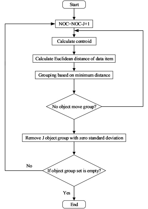
Table 2Algorithm overview of SOM optimized by PSO

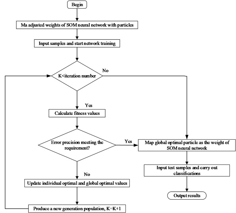
Step 1: Initialize particle swarm:

Initialize the velocity vector and the position vector of each particles. Then initialize the individual optimal value and the global optimum value.

Step 2: Express the SOM superior neighborhood

It determines the optimized adjusted weights of neighbourhood nodes. The function of topological distance is measured between the neighbourhood neuron and the winning neuron during the training period.

Step 3: The adjusted weight is mapped by means of particle swarm. Then input the training sample starts training. While, the training value is less than the set value, calculate the fitness function.

Step 4: After calculating the fitness, if error reaches the set value, the global optimal particle is mapped to the adjusted weights of SOM neural network. Otherwise, update the individual optimal value and the global optimal value.

Step 5: According to the PSO algorithm, produce a new generation population for the next training cycle.

Step 6: Finally, the optimal adjusted weights are obtained, with which the input testing samples are fed into the SOM neural network for fault classification test.

The fitness function is a main basis criteria that PSO algorithm guides the search engines. It was very important to construct the suitable fitness function for the optimization function. In this work, the classification accuracy of SOM in neural network was selected for the fitness function given in Fig. 3.

Algorithm overview. The deep learning process of the SOM neural network, weights the superior neighborhood particles directly affect the accuracy of samples. So, the PSO algorithm is used to optimize the weights of SOM neural network. This makes the weights of superior neighborhood particles achieve the optimal value. The various steps of PSO optimized the SOM neural network.

Fig. 3Flow chart of PSO optimized SOM

2.4. Semantic classifications

The DeepLab convolutional neural network (DL-CNN) semantically segment the image data to identify the bio-physical land coverage (crops, grass, and broad-leaved forest), socio-economic land usage (agriculture) and distinguish the crop types for spatial and territorial analyses. The major drawbacks of the existing methods include lack of end-to-end training, fixed size input and output, small/restricted field of view, low performance time consuming [31]. The combination of deep CNN with the conditional random field will overcome the existing drawbacks and yield in-depth segmentation maps.

The following concepts are important in the context of CNN:

The change detection is carried out using the deep learning classifier. Deep learning is primarily about neural networks, where a network is an interconnected web of nodes and edges. Neural nets were designed to perform complex tasks. Neural nets are highly structured networks and has three kinds of layers-an input, and so called hidden layers, which refer to any layers between the input and the output layers.

(i) Initialization-Xavier initialization to achieve convergence.

It is important to achieve convergence. We use the Xavier initialization. With this, the activations and the gradients are maintained in controlled levels, otherwise back-propagated gradients could vanish or explode.

(ii) Activation function- leaky rectifier linear unit for non-linearly transforming the data which achieve better results than the more classical sigmoid, or hyperbolic tangent functions, and speed up training.

(iii) DeepLabv2 (ResNet-101) Architecture- First, the Re-purposed ResNet-101 for semantic segmentation by dilated convolution, then the Multi-scale inputs with max-pooling to merge the results from all scales finally dilate the spatial pyramid pooling.

2.4.1. ResNet-101 feature extraction

The updated Deep-Lab neural network is called as the ResNet. This NN can better segment the objects at multiple scales, or either by multi-scale input processing. It is required to build a residual net variant of DeepLab by adapting the state-of-art ResNet image classification DCNN, achieving better semantic segmentation performance [32]. The identity mapping of ResNet-101 has similar effect as hyper-column features, which exploits the features from the intermediate layers to better localized boundaries. So, that the changes in the map are easily localized. Pre-trained ResNet-101 networks adapt them to the semantic segmentation task. The hypercolumn is introduced at the given input location, as the output of CNN are stacked into one vector. However, it includes not just an edge detector but for semantic units.

Fig. 4ResNet-101 feature extraction

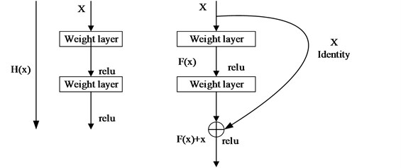
The desired underlying mapping can be denoted as $H (x)$ , we let the stacked nonlinear layers fit another mapping of $F (x) = H (x) - x$ , where $H (x)$ is any desired mapping.

The original mapping is recast into: $F (x) + x$ .

It is easier to optimize the residual mapping than to optimize the original, unreferenced mapping. For extreme, if an identity mapping was optimal, it would be easier to push the residual to zero than to fit an identity mapping by a stack of nonlinear layers given in Fig. 4.

The formulation of $F (x) + x$ can be realized by feed forward neural networks with “shortcut connections”.

2.4.1.1. Training of image in ResNet

Training and testing are two common concepts in machine learning. Training consists in learning a relation between data and attributes from a fraction of the training dataset, and testing consists in testing predictions of this relation on another part of the dataset. In image processing, training and testing is used for classifying pixels in order to segment different objects. The most common example was the classifier, as the user selects the pixels according to the interest, the classifier trained the set of pixel and then the remainder of the pixels are recognized to one of the classes by the classifier.

2.4.1.2. Mathematical formulation

In the training phase, the DNN with large amount of data are supplied for optimal convolutional weight settings to reduce the network error. To reach global minima, this phase needs many optimization rounds and also this is time consuming. Deep learning was an NN, in which the network is interconnected with nodes and edges. Neural nets are the highly structured networks which perform the complex tasks with three kinds of layers as an input, the hidden layer and an output layer. A DeepLabv2 (ResNet-101) are used in the proposed approach. Each layer can be defined as:

26

F^{j} (w_{j}, b_{j}) = δ (w_{j} * F^{j - 1} (w_{j - 1}, b_{j - 1}) + b_{j}),

where $j =$ [1, 2,…, 3], $w_{j}$ and $b_{j}$ represents the weight and the biases network, $F^{j} (w_{j}, b_{j})$ is the $j$ th layer output, $w_{j}$ is the weight with convolution size $m_{j - 1} \times m_{j} \times k_{j} \times k_{j}$ , where $k_{j}$ is the filter size of $j$ and $m_{j}$ is the amount of feature maps and function $δ$ denotes activation function.

The detailed information features include enduring crops, lines of trees, rivers, irrigation canals and grassland borders are extracted with the trained deep lab feature extractor. A loss function is formed during the training process. The loss function must be minimized to train the CNN accurately. The training phase is the stage with large number of data for searching the optimal convolutional weights to minimize the error. This phase is time-consuming and requires many rounds of optimization to reach global minima. An optimization algorithm is used to find a local minimum of a function, which overcome the drawback of the existing gradient descent.

2.5. Convolution neural network (CNN)

CNN is known to be a multilayer perceptron, which is used for identification of two-dimensional image formation. It is mainly classified into input layer, sample layer, convolutional layer and output layer [33]. The neurons parameter of CNN is set to be same, as sharing of weights. Each neuron forms same convolutional kernels to deconvolution of images.

2.5.1. Supervised classification with convolutional neural networks

Consider the two bands from Sentinel-1A scenes and the 6 bands from four Landsat 8 scenes from CNN with input feature vector. The traditional CNNs (2-D) of the image provide higher overall accuracy than per pixel-based approach. The CNN consists of two convolutional layers and these layers are followed by max pooling layer and the fully connected layer.

Rectified linear unit (ReLU) is used. It is most popular and efficient activation functions for deep NNs. There are advantages of using ReLU such as biological plausibility, efficient computation, and gradient propagation [34]. Consequently, the function of ReLU is faster and effective for the training process of CNNs than sigmoid function. In this function, there are 5 CNNs and each of the CNNs has the same convolution and max-pooling structure but differs in the trained filters and number of neurons in the hidden layer given in Fig. 5.

2.5.2. Network architecture

The CNNs flatten the input before applying the weights. It operates directly on the images. The filters are moved across the image left to right, top to bottom as if scanning the image and weighted sum of products are calculated between the filter and subset of the image. Therefore, these functioning are then passed through various other operations like non-linear activations and pooling.

Fig. 5Architecture of convolutional neural network

2.5.2.1. Input layer

The input layer specifies the image size. These layers relate to the height, width and channel size of input image.

2.5.2.2. Convolutional layer

The convolutional layer is mainly used for feature extraction of corresponding images. It captures the low-level image features as corners, edges and lines. Moreover, the training method uses the height and the width of filter, for scanning of images. It also determines the number of feature maps. It can be calculated as:

27

h_{j}^{n} = m a x (0, \sum_{k = 1}^{k} h k^{n - 1} * W_{k j}^{n}),

where, $h_{j}^{n}$ denotes the output feature map, $h k^{n - 1}$ is the input feature map and $k$ is the kernel function.

2.5.2.3. Batch normalization layer

The batch normalization is mainly used to improve the generalization. It normalizes the output of a convolutional layer before the non-linear layer. It normalizes the gradients propagation and the activation through a network, thus it makes the training an easier one. This layer speeds up the training functions and reduce sensitivity of network initialization. Calculate the average between training images for every channel and each pixels:

28

{\overset{˘}{x}}_{i j k} = \frac{1}{N} \sum_{n = 1}^{N} {x^{(n)}}_{i j k},

where ${\overset{˘}{x}}_{i j k}$ is pixel value, $k$ is the kernel function, $N$ number of input data, ${x^{(n)}}_{i j k}$ pixel value of channel $k$ and address ( $i, j$ ). For subtracting the average pixel value in the area of $P_{i j}$ from pixels of input image.

Average:

29

{\bar{x}}_{i j} = \frac{1}{H^{2}} \sum_{(p, q) \in p_{i, j}} x_{i} + p, j + q .

Weighted average:

30

{\bar{x}}_{i j} = \sum_{(p, q) \in p_{i j}} w_{p q} x_{i} + p, j + q,

where $H^{2}$ is the average value of pixel, pixel value ${\overset{˘}{x}}_{i j k}$ , $W$ is the weight.

2.5.2.4. ReLU layer

It is a very common activation function in the network. It is a very popular activation function in recent times.

It is a very popular activation function in recent times as:

31

f (x) = m a x (0, x) .

It can be used for modelling the real value.

2.5.2.5. Pooling layer

The pooling layer is important for scene classification and detection. The pooling values are unchanged, if the feature value is little bit changed. The pooling values is unchanged, if the feature value is little bit changed. The down-sampling in the convolutional layer reduce the spatial size and the redundant function of feature map and spatial layer respectively. The one way of down-sampling is the max pooling, in which it creates max pooling layer. It reduces the size of input or output to next layer.

Max pooling: Using the maximum value from $H^{2}$ pixels in the area. The standard way is represented as:

32

u_{i j k} = M a x_{p, q \in P {}_{i, j}} z_{p q k},

where; $P_{i j}$ denotes the set of pixels included the area, the pixel value $u_{i j k}$ is obtained by using $H^{2}$ pcs of the pixel value with every $K$ channels.

Average pooling: Using the average value from the $H^{2}$ pixels in the area:

33

u_{i j k} = \frac{1}{H^{2}} \sum_{(p, q) \in p_{i, j}} z_{p q k},

where, $H^{2}$ is the average value of pixel, $p_{i j}$ .

LP pooling is the common way including average pooling and the maximum pooling. The LP pooling can be represented as:

34

u_{i j k} = {(\frac{1}{H^{2}} \sum_{(p, q) \in p_{i, j}} {z^{p}}_{p q k})}^{1 / p} .

when $p =$ 1, it works on the average pooling.

When $p = \infty$ , it works on the Max pooling.

2.5.2.6. Fully connected layer

It mostly is used for removing the constraints and provides better summarizing information from low level layer. It connects all the corresponding neurons in the preceding layer. The fully connected layer combines the features of image for classification of images. Therefore, the size of output classes is same as that of fully connected data.

2.5.2.7. Softmax layer

The softmax layer normalizes the output of the fully connected layer. The output of the layer consists of positive numbers, which sums to one.

Classification layer. This layer makes the probabilities returned to the activation function for each input of the classes and then compute the loss.

2.6. Post processing and geospatial analysis

To improve the quality of the resulting map, we developed several filtering algorithms, based on the available information on quality of input data and fields boundaries. The final level of data processing provides data fusion with multisource heterogeneous information, in particular, statistical data, vector geospatial data, socio-economic information, and so on. It allows interpreting the classification results, solving applied problems for different domains, and provide support information for decision makers. For example, classification map coupled with area frame sampling approach can be used to estimate crop areas.

2.6.1. Accuracy assessment

Finally, the segmentation results show the land use and the land cover change, the forest and the vegetation change, urban change, wetland, and environmental change. The quality can be predicted with the resultant post-processing and geospatial analysis. The spatial filtering and sampling techniques are used in the resultant image to progress the quality.

3. Experimental result and discussion

The proposed work is implemented by using MATLAB 2017, a programming software. It compares the result with the Landsat public dataset. This dataset used to perform the semantic segmentation techniques in multispectral images. The scene is collected mostly in 22 Oct 2014, it includes a multispectral scenes with OLI and TIRS sensor. The Landsat public dataset having 12 spectral bands whose spatial dimensions are 500×500 pixels. The longitude of the dataset is 85.86664 (in degree) and latitude of 22.71835 (in degree). Our proposed method is compared with the prevailing method such as naïve Bayesian, SVM, KNN, RF, ENN.

Table 3Atmospheric parameters

Sensor type	Date	Time	Upwelling radiance	Down-welling radiance
Landsat 5 TM	13 Nov 2010	14.57	0.72	1.20
Landsat 5 TM	31 Dec 2010	14.57	0.58	0.97
Landsat 7 ETM+	21 Nov 2010	15.00	0.18	0.31
Landsat 7ETM+	23 Feb 2016	15.09	0.11	0.20
Landsat 8 TIRS	4 June 2015	15.06	0.91	1.52
Landsat 8 TIRS	29 May 2013	15.09	0.72	1.22
Landsat 8 PDS	22 Oct 2014	4.37	0.10	1.21

In this study, the estimation of the atmospheric parameters (transmittance, upwelling and down-welling radiance) of TM Landsat 5, Landsat 7 ETM+ and the Landsat 8 TIRS have been done through the NASA’S atmospheric parameters calculator. The tools used in the National Centers are modelled with the atmospheric global profiles incorporated by a particular date, time and the locations of inputs. Through this tool, the atmospheric profile of the study area has been simulated to the conditions through the satellite overpass time. The proposed sensor compared with other existing sensor types are based on its radiance and time [35]. The atmospheric transmittance with upwelling and down welling radiance used in the study was represented in Table 3.

3.1. Input database

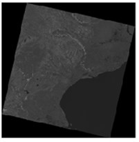
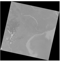
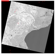
The multispectral remote sensing (RS) images are considered as a database for the proposed framework. In the proposed work, we use agriculture image band (2, 5, 6) are taken from the Landsat public dataset. These bands are given as input to the proposed automatic semantic segmentation technique given in Fig. 6.

Fig. 6Input image: a) band 2, b) band 5, and c) band 6

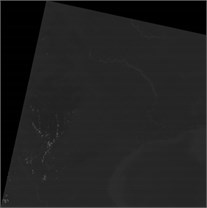
a)

b)

c)

3.2. Pre-processing

The pre-processing steps such as radiometric calibration, atmospheric correction, and mosaicking are performed on the image, to obtain the detailed information about the RS images.

3.2.1. Radiometric calibration and atmospheric correction

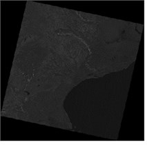
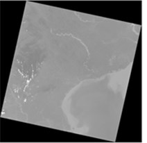
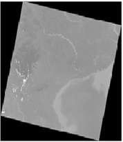
The key objective of radiometric correction was to recover the true radiance or the reflectance of the target. Moreover, it was used to increase the visual appearance of the image in Fig. 7. It avoids the radiometric errors, while geometric correction removes the geometric distortion from the images.

Fig. 7Radiometric calibration of: a) band 2, b) band 5, and c) band 6

a)

b)

c)

3.2.2. Atmospheric correction

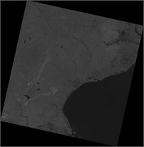
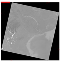
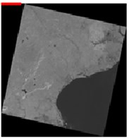
It was mainly used for removing effects of atmosphere on reflectance value in the solar radiation reflected from earth’s surface. The atmospheric correction was not needed for single scene data but it is essential while comparing multiple scenes. It reduces scattering and the absorption effect from the atmosphere.

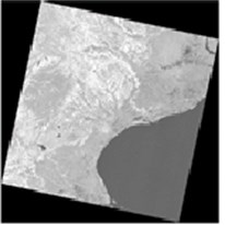
Dark object subtraction. The DOS, an image based method is to reduce haze component caused by means of additive scattering from the remote sensing data. As, the DOS method pursuits each band for darkest pixel value. Moreover, the scattering was removed by means of subtracting the value from each pixel in each band in Fig. 8.

Fig. 8Atmospheric correction of: a) band 2, b) band 5, and c) band 6

a)

b)

c)

3.2.3. Mosaicing

Mosaicing combines multiple individual images into a single scene. So, the scene is scanned part by part producing split image. After the analysis, combine the processed image to get complete final image. Methods for mosaicing of multispectral image is given below.

3.2.3.1. Feature extraction

Features of the two input images are to be matched. The images are taken inside the patches for match the input images. Those image patches are grouped and considered as the pixel in the image. Then match the pixel of each images by patch matching method to obtain matched images.

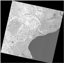
Harris corner detector. The corner detector method mainly matches the corresponding points of the consecutive agricultural image frames by tracking equally the corners and edges between the frames given in Fig. 9. This algorithm is quietly more desirable detector by means of detection and repeatability rate with more computation time.

Fig. 9Harris corner detector of: a) band 2, b) band 5, and c) band 6

a)

b)

c)

3.2.3.2. Image registration

It mainly aligns two images by same or different time or at different view point. For the image registration, we have to regulate the geometric transformation that arranges the images based on the reference image represent in Fig. 10.

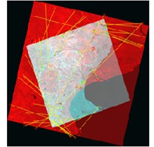
3.2.3.3. Homographic computation

The homographic computation is the mapping the space between two images of the same scene. It was mainly used wrapping multiple images to produce full image view. For the homographic detection method, we use RANdom sample consensus (RANSC) algorithm. The computed image is represented in Fig. 11.

Fig. 10Image registration of agriculture image

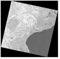
Fig. 11Homographic computation of agriculture image

3.3. Semantic segmentation using SOM

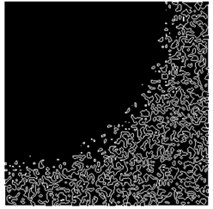
For the preprocessing stage, we use SOMs for the image segmentation and the subsequent restoration of missing data of satellite imaginary. It was a kind of neural network which was trained by means of unsupervised learning method, for providing low dimensional discretized representation of the input space of the training model. It was used to find the missed values and fill the gaps from the optical satellite imagery in Fig 12. Moreover, it segments the crop major types by means of semantic segmentation using SOM.

3.3.1. Clustering

Clustering is a process of separating a large class of objects into smaller classes together with the criterion for determining classes of the objects. The data elements as major crops with the high similarities are grouped up within a same cluster, while the less similarity of crops are grouped up in different clusters which was represented in Fig. 13.

Fig. 12Segmentation using SOM

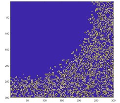
Fig. 13Clustering of classes

3.4. Automatic semantic classification using CNN

The DeepLab convolutional neural network (DL-CNN) semantically segments the image data to identify the bio-physical land coverage (crops, grass, and broad-leaved forest), socio-economic land usage (agriculture) and distinguish the crop types for spatial and territorial analyses. The major shortcomings of the existing methods include an end-to-end training manner, fixed size input & output, small/restricted field of view, low performance time consuming. The ResNet 101 CNN overcome the existing drawbacks and yield in-depth segmentation maps. The change detection was carried out by means of deep learning classifier. Moreover, it classifies the major crops accurately. Therefore, in our work, it classifies the major crops such as sugar beet, soya beans, rice, maize and the wheat given in Fig. 14.

In a proposed scenario, the resulting classification is detected by major-to-medium changes interfere. To evaluate the binary change detection methods, the following measures are computed: true positives (TP), true positive rate (PTP = TP/N1 × 100), true negatives (TN) and true negative rate (PTN = TN/N0×100), correct classification rate or overall accuracy (PCC = (TP + TN)/(N0 + N1) × 100), and error rate (PE = (FP + FN)/(N0 + N1) × 100), False Negative rate (FNR = FN/condition positive), PCC, kappa (K = observed accuracy-chance agreement/1-chance agreement), general precision (precision = TP/TP+FP). The proposed method related to the other classifier is SVM [36], RF [37], ENN and NN classifiers. The proposed method achieves the overall accuracy greater than 85 %. The results for the Evaluation Metrics over Up-to-date Methods on Dataset are shown in Table 4.

Fig. 14ResNet 101 convolution neural network

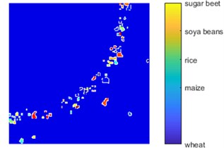
Table 4Evaluation metrics over state-of-the-art methods on dataset

Metrics/method	SVM	RF	ENN	NN	Proposed method
TP	105	134	145	143	270
FP	200	132	121	139	240
TN	15.55	5	131	135	30
FN	9.9	7	17	19	30
Precision	87.312	96.4	82.64	83.11	94.0
Recall	79.432	95.0	88.12	87.97	100
F-Measure	81.156	96.4	88.98	81.34	97.3
TNR	86.074	96.4	80.98	81.23	66.67
FPR	65.987	91.3	65.2	44.9	33.0
FNR	98.990	86.3	79.98	87.91	88.8
PCC	77.487	81.0	79.12	82.32	82.94
kappa	89.012	91.5	80.7	69.7	80.9
Overall accuracy (%)	76.181	82.0	80.89	74.99	95
Overall error	6	1.95	5	4.99	4.7

In our proposed framework, the resulting segmentation method is detected by major-to-medium changes interfere. To evaluate the evaluation metrics over state-of-the-art segmentation algorithms on dataset, the following measures are computed: true positives (TP), true positive rate (PT P = TP/N1 × 100), true negatives (TN) and true negative rate (PT N = T N/N0×100), correct classification rate or overall accuracy (PCC = (TP + TN)/(N0 + N1) × 100), and error rate (PE = (FP + FN)/(N0 + N1) × 100), False Negative rate (FNR=FN/condition positive), PCC, kappa (K = observed accuracy-chance agreement/1-chance agreement), general precision (precision = TP/TP+FP). The proposed segmentation method is compared with the other existing segmentation system as (1) Kampffmeyer et al. [38]. In [38] authors introduced the simple convolutional neural network for semantic segmentation of land cover in RS images. It only considers the true positive, negative and the accuracy, but it fails to calculate other parameters. The results of the existing work show, that the overall classification accuracy as 87 %, corresponding F1- score for the small object is 80.6 %. (2) Zhang et al. [39] proposed a multi-scale feature fusion method based on a weighted across-scale combination strategy to generate the saliency map using adaptive threshold segmentation method. It only considers the true positive, negative, precision, recall and OA, but it fails to calculate other parameters. The results of the existing work show, that the overall classification accuracy of 75.26 %, corresponding F1- score for the small object is 79.8 %, precision is 51 % and had a high system complexity. (3) Leichtle et al. [40] projected a multiresolution segmentation. The performance of segmentation algorithms is essential to identify effective segmentation methods and optimize their parameters. The two measures are calculated such as precision, recall, that can indicate segmentation quality in both geometric and arithmetic respects. It considers true and false values, precision and recall as 94 % and 95 % respectively with OA of 94 %, but this method fails to achieve better segmentation results. (4) Henry et al. [41], proposes Fully-Convolutional Neural Network (FCNN) semantic segmentation in SAR images. It has two approaches, binary segmentation and regression, intolerant and tolerant to prediction errors, respectively. The FCNN model shows promising comparative results such as true positive and negative values with precision of 62.27 %, recall of 60 % and OA 84.5 %. But, these methods have a lack of some important significant parameters, such as lack of providing accurate accuracy assessment, correct feature extraction and classifications. It cannot predict correct change detection results. Moreover, those work provides high error rates according to such parameters. Therefore, our proposed method calculates all metrics the based-on segmentation of RS images. As a result, our novel method achieves the overall accuracy of 95 %, as compared to existing methods. The results for the Evaluation Metrics over state-of-the-art segmentation algorithms on dataset are shown in Table 5.

Table 5Evaluation metrics over state-of-the-art segmentation algorithms on dataset

Metrics/Method	Kampffmeyer et al.	Zhang et al.	Zhang et al.	Henry et al.	Proposed method
TP	128	255	150	160	270
FP	96	255	120	58.9 %	240
TN	16	–	30	41.85	30
FN	–	–	25	40.69	30
Precision	–	51 %	94 %	62.27	94.0 %
Recall	–	88 %	95 %	60.00 %	100 %
F-Measure	80.6 %	79.8 %	80 %	81 %	97.3 %
TNR	–	85.2 %	–	–	66.67
FPR	–	89.1 %	–	–	33.0
FNR	–	–	–	–	88.8
PCC	–	–	87 %	–	82.94
kappa	–	–	87 %	–	80.9 %
Overall accuracy (%)	87 %	75.26 %	94 %	84.5 %	95 %
Overall error	–	13.52	3	5	4.7

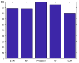
Fig. 15 shows the performances of overall Accuracy for proposed classifier. The above graph shows better accuracy than the existing technique. The proposed CNN classifier classifies the multispectral data. The OA of the proposed method is compared with the SVM, NN, ENN and RF classifier. Therefore, the new method attains better accuracy of 95 % which is greater than other existing classifiers.

Fig. 15Performance of overall accuracy

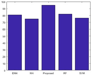
Fig. 16Performance of precision

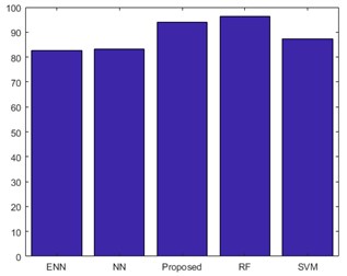
Fig. 16 shows the performances of precision for proposed classifier. The above graph shows better precision value than the existing technique. The precision considers the true positive and the true negative values. The precision of the proposed method is compared with SVM, NN, ENN and RF classifier. Therefore, the proposed system achieves better precision rate than the other existing classifiers.

Fig. 17 shows the performances of recall for proposed classifier. The above graph shows better recall value than the existing technique. The recall also considers the true positive and the true negative values of the proposed CNN. The recall of the proposed method is compared with SVM, NN, ENN and RF classifier. Therefore, the proposed system attains better recall rate than other existing classifiers.

Fig. 17Performance of recall

4. Conclusions

In this manuscript, we have projected an automatic semantic segmentation for land cover and crop type classifications using multispectral satellite imagery. The RS images are high resolution images which can be used for agricultural and land cover classifications. Due to the large dimension of feature space, the conventional feature extraction techniques represent a progress of issues when handling huge size information e.g., computational cost, processing capacity and storage load. To overcome the existing drawback, we propose an automatic semantic segmentation without losing the significant data. In this paper, we use SOMs for segmentation purpose. Moreover, we proposed the PSO optimization algorithm used for finding the cluster limitations directly from the SOMs. In contrast, we propose the deep residual network to achieve faster training process. Deep Residual Networks have been proven to a very effective model on RS image classification. Furthermore, the main purpose of the work is to achieve the overall accuracy greater than 85 % (OA > 85 %). So, we use a CNN, which outperforms better classification of certain crop types and yield the target accuracies which is more than 85 % for all major crops. The foremost advantage of CNNs, enable to construct hierarchy of local and sparse features derived from the spectral and temporal profiles while other classifiers use a global transformation of features. Few objects in the final classification map is provided by CNNs are smoothed and misclassified.

References

Drusch M., Bello D., Colin O., Fernandez V. Sentinel-2: ESA’s optical high-resolution mission for GMES operational services. Remote Sensing of Environment, Vol. 120, 2012, p. 25-36.

Publisher
Roy D. P., Welder M. A., Loveland T. R. Landsat-8: Science and product vision for terrestrial global change research. Remote Sensing of Environment, Vol. 145, 2014, p. 154-172.

Publisher
Zhang J. Multi-source remote sensing data fusion: status and trends. International Journal of Image and Data Fusion, Vol. 1, Issue 1, 2010, p. 5-24.

Publisher
Chen Y., Zhao X., Jia X. Spectral-spatial classification of hyperspectral data based on deep belief network. IEEE Journal of Selected Topics in Applied Earth Observations and Remote Sensing, Vol. 8, Issue 6, 2015, p. 2381-2392.

Publisher
Zhang F., Du B. Saliency-guided unsupervised feature learning for scene classification. IEEE Transactions on Geoscience and Remote Sensing, Vol. 53, Issue 4, 2015, p. 2175-2184.

Publisher
Hussain M., Chen D., Cheng A., Wei H., Stanley D. Change detection from remotely sensed images: From pixel based to object-based approaches. ISPRS Journal of Photography and Remote Sensing, Vol. 80, 2013, p. 91-106.

Publisher
Skakun S., Kussai N., Basarah R. Restoration of missing data due to clouds on the optical satellite imagery using neural networks. Sentinel-2 for Science Workshop, 2014.

Search CrossRef
Neubert M., Heroldf H., Minel G. Evaluation of remote sensing image segmentation quality-further results and concepts. International Archives of Photogrammetry, Remote Sensing and Spatial Information Sciences 36.4/C42, 2006.

Search CrossRef
Khatami R., Mountrakis G., Stehman S. V. A meta-analysis of remote sensing research on supervised pixel-based land-cover image classification processes: general guidelines for practitioners and future research. Remote Sensing of Environment, Vol. 177, 2016, p. 89-100.

Publisher
Han M., Zhu X., Yao W. Remote sensing image classification based on neural network ensemble algorithm. Neurocomputing, Vol. 78, Issue 1, 2012, p. 133-138.

Publisher
Lavreniuk M. S., Skakun S. V., Shelestov A. J. Large-scale classification of land cover using retrospective satellite data. Cybernetics and Systems Analysis, Vol. 52, Issue 1, 2016, p. 127-138.

Publisher
Chen Y., Lin Z., Zhao X., Wang G., Gu Y. Deep learning-based classification of hyperspectral data. IEEE Journal of Selected Topics in Applied Earth Observations and Remote Sensing, Vol. 7, Issue 6, 2014, p. 2094-2107.

Publisher
Zhao W., Du S. Learning multiscale and deep representations for classifying remotely sensed imagery. ISPRS Journal of Photogrammetry and Remote Sensing, Vol. 113, 2016, p. 155-165.

Publisher
Kussul N., Lavreniuk N., Shelestov A., Yailymov B., Butko D. Land cover changes analysis based on deep machine learning technique. Journal of Automation and Information Sciences, Vol. 48, Issue 5, 2016, p. 42-54.

Publisher
Gallego F. J., Kussul N., Skakun S., Kravchenko O., Shelestov A., Kussul O. Efficiency assessment of using satellite data for crop area estimation in Ukraine. International Journal of Applied Earth Observation and Geoinformation, Vol. 29, 2014, p. 22-30.

Publisher
Su T. Efficient paddy field mapping using Landsat-8 imagery and object-based image analysis based on advanced fractel net evolution approach. GIScience and Remote Sensing, Vol. 54, Issue 3, 2017, p. 354-380.

Publisher
Maggiori E., Tarabalka Y., Charpiat G., Alliez P. Convolutional neural networks for large-scale remote-sensing image classification. IEEE Transactions on Geoscience and Remote Sensing, Vol. 55, Issue 2, 2017, p. 645-657.

Publisher
Bargoti S., Underwood J. P. Image segmentation for fruit detection and yield estimation in apple orchards. Journal of Field Robotics, Vol. 34, Issue 6, 2017, p. 1039-1060.

Publisher
Mccool C., Perez T., Upcroft B. Mixtures of lightweight deep convolutional neural networks: applied to agricultural robotics. IEEE Robotics and Automation Letters, Vol. 2, Issue 3, 2017, p. 1344-1351.

Publisher
Pei W., Yao S., Knight J. F., Dong S., Pelletier K., Rampi L. P., Wang Y., Klassen J. Mapping and detection of land use change in a coal mining area using object-based image analysis. Environmental Earth Sciences, Vol. 76, Issue 3, 2017, p. 125.

Publisher
Ma L., Li M., Ma X., Cheng L., Liu Y. A review of supervised object based land cover image classifications. ISPRS Journal of Photography and Remote Sensing, Vol. 130, 2017, p. 277-293.

Publisher
Li He, Chen Z. X., Jiang Z. W., Wu W. B., Ren J. Q., Liu Bin, Tuya H. Comparative analysis of GF-1, HJ-1, and Landsat-8 data for estimating the leaf area index of winter wheat. Journal of Integrative Agriculture, Vol. 16, Issue 2, 2017, p. 266-285.

Publisher
Zhu Z. Change detection using Landsat time series: a review of frequencies, preprocessing, algorithms, and applications. ISPRS Journal of Photogrammetry and Remote Sensing, Vol. 130, 2017, p. 370-384.

Publisher
Gerace A., Montanaro M. Derivation and validation of the stray light correction algorithm for the thermal infrared sensor onboard Landsat 8. Remote Sensing of Environment, Vol. 191, 2017, p. 246-257.

Publisher
Bernardo N., Watanabe F., Rodrigues T., Alcântara E. Atmospheric correction issues for retrieving total suspended matter concentrations in inland waters using OLI/Landsat-8 image. Advances in Space Research, Vol. 59, Issue 9, 2017, p. 2335-2348.

Publisher
Mwaniki M. W., Kuria D. N., Boitt M. K., Ngigi T. G. Image enhancements of Landsat 8 (OLI) and SAR data for preliminary landslide identification and mapping applied to the central region of Kenya. Geomorphology, Vol. 282, 2017, p. 162-175.

Publisher
Honjo T., Tsunematsu N., Yokoyama H., Yamasaki Y., Umeki K. Analysis of urban surface temperature change using structure-from-motion thermal mosaicing. Urban Climate, Vol. 20, 2017, p. 135-147.

Publisher
Chen B., Xiao X., Li X., Pan L., Doughty R., Ma J., Dong J., Qin Y., Zhao B., Wu Z., Sun R. A mangrove forest map of China in 2015: analysis of time series Landsat 7/8 and sentinel-1A imagery in google earth engine cloud computing platform. ISPRS Journal of Photogrammetry and Remote Sensing, Vol. 131, 2017, p. 104-120.

Publisher
Zolotov D. V., Chernykh D. V., Biryukov R. Y., Pershin D. K. Changes in the activity of higher vascular plants species in the Ob plateau landscapes (Altai Krai, Russia) due to anthropogenic transformation. Climate Change, Extreme Events and Disaster Risk Reduction, 2018, p. 147-157.

Publisher
Weisberg P. J., Dilts T. E., Baughman O. W., Meyer S. E., Leger E. A., Van Gunst K. J., Cleeves L. Development of remote sensing indicators for mapping episodic die-off of an invasive annual grass (Bromus tectorum) from the Landsat archive. Ecological Indicators, Vol. 79, 2017, p. 173-181.

Publisher
Marmanis D., Schindler K., Wegner J. D., Galliani S., Datcu M., Stilla U. Classification with an edge: Improving semantic image segmentation with boundary detection. ISPRS Journal of Photogrammetry and Remote Sensing, Vol. 135, 2018, p. 158-172.

Publisher
Zhan Y., Wang J., Shi J., Cheng G., Yao L., Sun W. Distinguishing cloud and snow in satellite images via deep convolutional network. IEEE Geoscience and Remote Sensing Letters, Vol. 14, Issue 10, 2017, p. 1785-1789.

Publisher
Long Y., Gong Y., Xiao Z., Liu Q. Accurate object localization in remote sensing images based on convolutional neural networks. IEEE Transactions on Geoscience and Remote Sensing, Vol. 55, Issue 5, 2017, p. 2486-2498.

Publisher
Yu X., Wu X., Luo C., Ren P. Deep learning in remote sensing scene classification: a data augmentation enhanced convolutional neural network framework. GIScience and Remote Sensing, Vol. 54, Issue 5, 2017, p. 741-758.

Publisher
Isaya Ndossi M., Avdan U. Application of open source coding technologies in the production of land surface temperature (LST) maps from Landsat: a PyQGIS plugin. Remote Sensing, Vol. 8, Issue 5, 2016, p. 413.

Publisher
Sokolova M., Japkowicz N., Szpakowicz S. Beyond accuracy, F-score and ROC: a family of discriminant measures for performance evaluation. Australasian Joint Conference on Artificial Intelligence, 2006, p. 1015-1021.

Publisher
Chapi K., Singh V. P., Shirzadi A., Shahabi H., Bui D. T., Pham B. T., Khosravi K. A novel hybrid artificial intelligence approach for flood susceptibility assessment. Environmental Modelling and Software, Vol. 95, 2017, p. 229-245.

Publisher
Kampffmeyer M., Salberg A. B., Jenssen R. Semantic segmentation of small objects and modeling of uncertainty in urban remote sensing images using deep convolutional neural networks. Computer IEEE Conference on Vision and Pattern Recognition Workshops, 2016, p. 680-688.

Publisher
Zhang L., Qiu B., Yu X., Xu J. Multi-scale hybrid saliency analysis for region of interest detection in very high resolution remote sensing images. Image and Vision Computing, Vol. 35, 2015, p. 1-13.

Publisher
Zhang X., Feng X., Xiao P., He G., Zhu L. Segmentation quality evaluation using region-based precision and recall measures for remote sensing images. ISPRS Journal of Photogrammetry and Remote Sensing, Vol. 102, 2015, p. 73-84.

Publisher
Henry C., Azimi Sm, Merkle N. Road segmentation in SAR satellite images with deep fully-convolutional neural networks. Computer Vision and Pattern Recognition, arXiv:1802.01445, 2018.

Publisher

Cited by

Progress in Pattern Recognition, Image Analysis, Computer Vision, and Applications

Sebastián Moreno | Javier Lopatin | Diego Corvalán | Alejandra Bravo-Diaz

(2025)

ESDINet: Efficient Shallow-Deep Interaction Network for Semantic Segmentation of High-Resolution Aerial Images

(2024)

Stealthy Adversarial Examples for Semantic Segmentation in Remote Sensing

Tao Bai | Yiming Cao | Yonghao Xu | Bihan Wen

(2024)

Ticino: A multi-modal remote sensing dataset for semantic segmentation

Mirko Paolo Barbato | Flavio Piccoli | Paolo Napoletano

(2024)

An improved semantic segmentation algorithm for high-resolution remote sensing images based on DeepLabv3+

Yan Wang | Ling Yang | Xinzhan Liu | Pengfei Yan

(2024)

A Novel Technique for Semantic Segmentation of Hyperspectral Images Using Multi-View Features

Reaya Grewal | Geeta Kasana | Singara Singh Kasana

(2024)

Geocomplexity Statistical Indicator to Enhance Multiclass Semantic Segmentation of Remotely Sensed Data with Less Sampling Bias

Wei He | Lianfa Li | Xilin Gao

(2024)

Semantic segmentation of agricultural images: A survey

Zifei Luo | Wenzhu Yang | Yunfeng Yuan | Ruru Gou | Xiaonan Li

(2024)

Weakly Supervised Remote Sensing Image Semantic Segmentation With Pseudo-Label Noise Suppression

Xiao Lu | Zhiguo Jiang | Haopeng Zhang

(2024)

A Lightweight High-Resolution Remote Sensing Image Cultivated Land Extraction Method Integrating Transfer Learning and SENet

Lin Li | Zhiwei Chen | Yangyang Ma | Lizhi Liu

(2024)

A Multispectral Remote Sensing Crop Segmentation Method Based on Segment Anything Model Using Multistage Adaptation Fine-Tuning

(2024)

Identification of Black Reef Shipwreck Sites Using AI and Satellite Multispectral Imagery

Alexandra Karamitrou | Fraser Sturt | Petros Bogiatzis

(2023)

The current state on usage of image mosaic algorithms

Bose Alex Lungisani | Caspar K. Lebekwe | Adamu Murtala Zungeru | Abid Yahya

(2022)

Joint alignment of the distribution in input and feature space for cross-domain aerial image semantic segmentation

(2022)

A review of deep learning methods for semantic segmentation of remote sensing imagery

Xiaohui Yuan | Jianfang Shi | Lichuan Gu

(2021)

Deep Learning Applications and Intelligent Decision Making in Engineering

Asha Gowda Karegowda | Devika G. | Geetha M.

(2021)

Deep Learning Spatial-Spectral Classification of Remote Sensing Images by Applying Morphology-Based Differential Extinction Profile (DEP)

Nafiseh Kakhani | Mehdi Mokhtarzade | Mohammad Javad Valadan Zoej

(2021)

Autonomous Crop Row Guidance Using Adaptive Multi-ROI in Strawberry Fields

Vignesh Raja Ponnambalam | Marianne Bakken | Richard J. D. Moore | Jon Glenn Omholt Gjevestad | Pål Johan From

(2020)

About this article

Received

23 March 2018

Accepted

07 May 2018

Published

30 June 2018

DOI

https://doi.org/10.21595/mme.2018.19840

Keywords

CNNs

deep learning (DL)

crop classification

landsat-8 remote sensing (RS)

self-organizing map (SOMs)

change detection (CD)

This is an open access article distributed under the Creative Commons Attribution License, which permits unrestricted use, distribution, and reproduction in any medium, provided the original work is properly cited.

Previous article in issue Previous

Research article

2024 02 23

Lightweight small target detection based on aerial remote sensing images

Muzi Li

Research article

2023 11 18

Target detection algorithm based on super- resolution color remote sensing image reconstruction

Zhihong Wang, Chaoying Wang, Yonggang Chen, Jianxin Li

Research article

2023 10 06

Application of optimized CNN algorithm in landslide boundary detection

Lili Wang, Yun Qiao

Research article

2023 01 30

An improved YOLOv5 algorithm for obscured target recognition

Zhizhan Lu, Ruili Wang, Yunfeng Jin, Chao Liang

J. K. Jadhav and R. P. Singh, “Automatic semantic segmentation and classification of remote sensing data for agriculture,” Mathematical Models in Engineering, Vol. 4, No. 2, pp. 112–137, Jun. 2018, https://doi.org/10.21595/mme.2018.19840

Copy Extrica

Copied to clipboard!

TY  - JOUR
DO  - 10.21595/mme.2018.19840
UR  - https://doi.org/10.21595/mme.2018.19840
TI  - Automatic semantic segmentation and classification of remote sensing data for agriculture
T2  - Mathematical Models in Engineering
AU  - Jadhav, Jagannath K.
AU  - Singh, R. P.
PY  - 2018
DA  - 2018/06/30
PB  - JVE International Ltd.
SP  - 112-137
IS  - 2
VL  - 4
SN  - 2351-5279
SN  - 2424-4627
ER  - 

Copy Ris

Copied to clipboard!

@article{Jadhav_2018,
	doi = {10.21595/mme.2018.19840},
	url = {https://doi.org/10.21595/mme.2018.19840},
	year = 2018,
	month = {jun},
	publisher = {{JVE} International Ltd.},
	volume = {4},
	number = {2},
	pages = {112--137},
	author = {Jagannath K. Jadhav and R. P. Singh},
	title = {Automatic semantic segmentation and classification of remote sensing data for agriculture},
	journal = {Mathematical Models in Engineering}
}

Copy Bibtex

Copied to clipboard!

[1]J. K. Jadhav and R. P. Singh, “Automatic semantic segmentation and classification of remote sensing data for agriculture,” Mathematical Models in Engineering, vol. 4, no. 2, pp. 112–137, Jun. 2018, doi: 10.21595/mme.2018.19840.

Copy IEEE

Copied to clipboard!

Jadhav, Jagannath K., and R. P. Singh. “Automatic Semantic Segmentation and Classification of Remote Sensing Data for Agriculture.” Mathematical Models in Engineering 4, no. 2 (June 30, 2018): 112–37. https://doi.org/10.21595/mme.2018.19840.

Copy Chicago

Copied to clipboard!

Automatic semantic segmentation and classification of remote sensing data for agriculture

Abstract

1. Introduction

2. Proposed methodology

2.1. Input database

2.2. Pre-processing

2.2.1. Radiometric calibration

2.2.2. Atmospheric correction

2.2.2.1. Dark-object subtraction (DOS)

2.2.3. Mosaicing

2.2.3.1. Feature extraction

2.2.3.2. Image registration

2.2.3.3. Homographic computation

2.3. Semantic segmentation using SOM (self organizing map)

2.3.1. Learning algorithm

2.3.1.1. Initializing the weights

2.3.1.2. Calculating the best matching unit (BMU)

2.3.1.3. Determine the best matching unit’s local neighbourhood

2.3.1.4. Adjusting the weights

2.3.2. Clustering

2.3.3. SOM neural network optimized by particle swarm optimization (PSO)

2.3.4. Training steps of PSO algorithm

2.4. Semantic classifications

2.4.1. ResNet-101 feature extraction

2.4.1.1. Training of image in ResNet

2.4.1.2. Mathematical formulation

2.5. Convolution neural network (CNN)

2.5.1. Supervised classification with convolutional neural networks

2.5.2. Network architecture

2.5.2.1. Input layer

2.5.2.2. Convolutional layer

2.5.2.3. Batch normalization layer

2.5.2.4. ReLU layer

2.5.2.5. Pooling layer

2.5.2.6. Fully connected layer

2.5.2.7. Softmax layer

2.6. Post processing and geospatial analysis

2.6.1. Accuracy assessment

3. Experimental result and discussion

3.1. Input database

3.2. Pre-processing

3.2.1. Radiometric calibration and atmospheric correction

3.2.2. Atmospheric correction

3.2.3. Mosaicing

3.2.3.1. Feature extraction

3.2.3.2. Image registration

3.2.3.3. Homographic computation

3.3. Semantic segmentation using SOM

3.3.1. Clustering

3.4. Automatic semantic classification using CNN

4. Conclusions

References

Cited by

About this article

Related Articles