The coherent sound field separation method combining compressive sensing

2.1. Plane equivalent source method near-field acoustic radiation calculation model

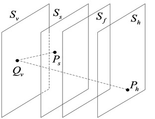
Setting the virtual sound sources on a plane, which has better convenience and versatility. As shown in Fig. 1, $S_v$ represents the virtual sound source plane, $S_s$ represents the sound source plane, $S_f$ represents a plane in the sound field, $S_h$ represents the holographic surface, $n$ represents the normal direction of the sound source outside the plane, $P_h$ is the sound pressure distribution on the holographic surface, and $P_s$ is the sound source plane Sound pressure distribution, $Q_v$ is the sound intensity of the virtual sound source.

Fig. 1A schematic diagram of Plane ESM

The sound pressure distribution on the holographic surface can be represented by the following integral equation:

where $g\left(\mathbf{r},{\mathbf{r}}_0\right)$ is the free space Green’s function from the virtual point source to the point which is on the holographic surface, $q_v\left({\mathbf{r}}_0\right)$ is the virtual point sound source intensity, $\rho$ is the medium density, $c$ is the sound speed, and $k$ is the wave number. The sound pressure on the actual sound source surface can be expressed in the following form after being discretized:

where $P_s$ is the sound source surface acoustic pressure column vector, $Q_v$ is the source strong column vector of the equivalent source sequence, and $G_{sv}$ is the sound pressure matching matrix between the equivalent source sequence and the sound source surface:

After the sound pressure on the holographic surface is discretized, it can be expressed as:

$P_h$ is the sound pressure column vector on the holographic surface, $Q_v$ is the source strong column vector of the equivalent source sequence, and $G_{hv}$ is the sound pressure matching matrix between the equivalent source sequence and the holographic surface:

The inversion formula for the virtual source strength is:

Further, the sound pressure of the actual sound source surface can be expressed as:

The sound pressure transfer matrix from the sound source surface to the holographic surface is expressed as:

Get the sound pressure $P_S$ on the sound source surface:

Knowing $L$ and $P_h\text{,}$ the sound pressure distribution on the sound source plane can be reconstructed. If know the sound pressure transfer matrix $L$ from the sound source plane $S_s$ to a certain plane $S_f$ in the sound field and the sound pressure $P_h$ on the holographic plane, the sound pressure distribution on any plane $S_f$ in the sound field can also be reconstructed.

2.2. Sparse representation model of acoustic pressure array signals

As shown in Fig. 2, on the holographic plane $S_h$, there is a regular array of $M$-element microphones. The sound source points are sparsely distributed on the sound source surface $S_s$. The sound source surface $S_s$ can be evenly divided into grid points so that the sound source points can be sparsely represented on the sound source surface [7].

Fig. 2Microphone array signal sampling model

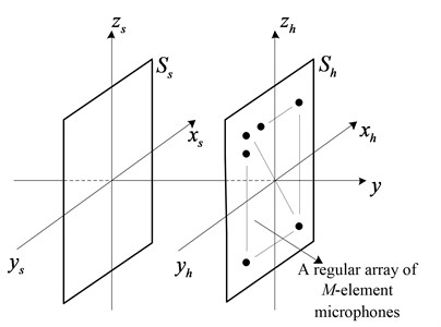
Fig. 3Sound source surface sparse representation

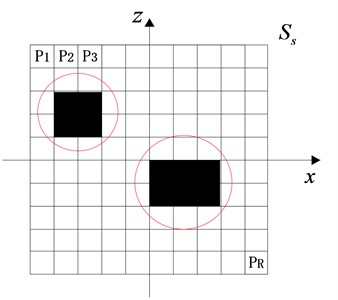
As shown in Fig. 3, the sound source surface $S_s$ is divided into $R$ areas. A solid area indicates that there is a sound source at that location, and a hollow area indicates that there is no sound source. A single sound source is often a small area element, which can be viewed as a collection of several point sources. The sound pressure signals received by the regularly distributed $M$-element microphone array is sparsely represented as:

In the formula, $y$ is an $M\times 1$ dimensional matrix, which represents the signal received by the microphone array. $A$ is an $M\times R$ dimensional matrix that represents the sensing matrix. $x$ is an $R\times 1$ dimensional matrix and represents a sound source signal containing position information, of which there are only $N\left(N\ll R\right)$ non-zero values. $\theta$ is the received noise signal.

2.3. A coherent sound field separation method combined with compression sensing

In the planar equivalent source near-field acoustic radiation model, the virtual sound source surface $S_v$ is discretized. The virtual sound source points are sparsely distributed on $S_v$. The transfer matrix in the plane ESM is directly used as a sensing matrix, and the matrix conforms to the Restricted Isometry Property (RIP) [8]. Firstly, the position of the virtual sound sources on the virtual sound source surface is obtained by orthogonal matching pursuit (OMP) algorithm, and then the near-field plane sound pressure distribution is reconstructed in combination with the known transfer matrix. In the plane rectangular coordinate system, the virtual sound source plane may be discretized into $I\times I$ uniform squares, and the microphones on the holographic surface may also be evenly spaced to facilitate calculation. The sound pressure transfer matrix from the sound source plane $S_s$ to a plane $S_f$ in the sound field can be expressed as:

This is the sensing matrix, $G_{vf}$ is the sound pressure matching matrix between the equivalent source sequence and a plane in the sound field:

Substituting Eq. (11) into Eq. (10) yields:

The presence of a noise signal will affect the accuracy of sound source localization, where $\theta$ is the noise signal, which is directly recorded by the array, so Eq. (13) can be written as:

According to the flow of the OMP reconstruction algorithm [9, 10], it is necessary to input the sensing matrix $L$, the observation vector $y$, and the signal sparsity $K$. In practice, a single virtual sound source is a small area element, which can be regarded as a collection of several point sources, so the input sparsity K can be approximated. Referring to the example of the OMP reconstruction algorithm given by Tropp [10], after knowing the relationship between the sampled value $M$ and the reconstruction success rate and the relationship between the signal sparsity $K$ and the reconstruction success rate, the sparsity $K$ can be determined.

After finding the sparse distribution $x^{\text{'}}$ of the virtual sound sources, the virtual sound sources are grouped, and those grouped together are grouped into the same group. As shown in Fig. 3, the same group is in the red circle. Assuming there are two coherent sound sources, the virtual sources are divided into two groups, one of which is selected to obtain a sparse distribution $x^{\text{'}\text{'}}$.

The transfer matrix is known to be calculated in combination with $x^{\text{'}}$ and $x^{\text{'}\text{'}}$:

Subtract the two equations to obtain the separated sound field on any near-field plane $S_f$ that is a distance $d$ from the actual sound source plane:

3.1. Discs vibration model

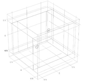
Sound radiation model shown in Fig. 4. Both discs have a radius of 0.05 m and a thickness of 0.008 m. Both materials are alloy structural steels. The central axis of the two discs is parallel to the $y$-axis, and the two discs are equally distributed along the $y$-axis. The coordinates of the center of the discs distributed are (0.2, 0, 0.2) and (–0.2, 0, –0.2). A 10 N excitation force is applied in the normal direction at the center of both discs at a frequency of 500 Hz.

Fig. 4Sound field three-dimensional model

3.2. Sound field holographic simulation imaging analysis

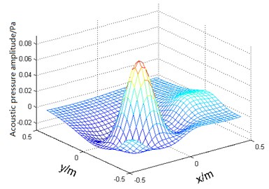
Fig. 5 shows the sound pressure distribution of an ideal sound field separated on a plane 0.1 m from the side of the discs. From the side of the disc 0.2 m on the plane, the sound pressure distribution shown in Fig. 6.

Fig. 5Sound pressure distribution of an ideal sound field separated

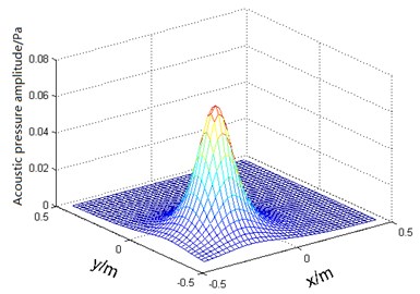
a)

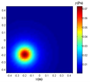
b)

A 11×11 array microphones are used to sample the sound pressure shown in Fig. 6. Divide the virtual sound source surface into 16×16 grids. At this time, according to the example of Tropp, when the sparsity $K$ is 22, there is good reconstruction success rate. When reconstructing the sound pressure distribution of the separated sound field in the plane of 0.1 m from the sound source plane, the plane is divided into 41×41 grids for sound pressure reconstruction.

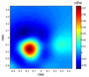
Use the method proposed in this paper to separate the composite sound pressure on the holographic surface. Fig. 7 shows the virtual sound sources distribution. Only the sound sources in the lower left red circle participate in the sound pressure reconstruction. The result of the calculation is shown in Fig. 8.

Fig. 6Plane sound pressure distribution at 0.2 m

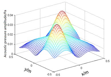
a)

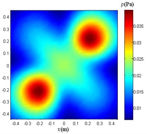
b)

Fig. 7Virtual sources distribution

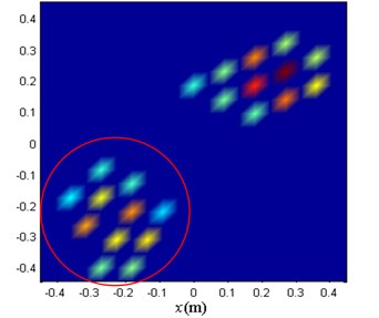
Fig. 8Sound field separation result graph

a)

b)

3.3. Results and discussion

The composite sound pressure shown in Fig. 6 is separated according to the method proposed in this paper. The results obtained are shown in Fig. 8. The coherent sound field is separated using the method proposed in this paper. The results obtained are good, and the sound source location is accurate, but there is a slight error in the local sound pressure value.

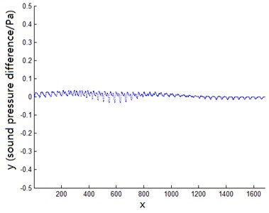
As shown in Fig. 9, a scatter plot is made for the difference between the calculated value and the theoretical value of the separated sound field, which is 41×41 points in total. The errors are all around zero. There are only little local errors, which is consistent with Fig. 8.

Fig. 9Sound pressure differences scatter plot