Fatigue life prognostic for medium-carbon steel based S-N curve computation and deep autoencoder

1. Introduction

Medium-carbon steel is the most common steel that widely used for critical components due to good resistance, strength, and machining ability. So, the research of medium-carbon reality is essential to the safety and reliability. Medium-carbon’s strength value is certain, but its fatigue life is influenced by the roughness and stress of structure. Therefore, it is vital to explore the influence of different roughness and stress on the fatigue life of medium-carbon steel [1].

For the study of the fatigue life of medium carbon steel, there are some existing methods: 1. Surface condition modification factor method. It considers the impact of roughness on fatigue life as a modification factor which can be achieved by statistical analysis. Then, the critical location's endurance limit is proportional to the endurance limit based on rotating cantilever bending fatigue testing [2]. 2. Stress concentration factor theory. It deems that the surface groove leads to a local stress concentration and the impact of roughness can be simplified as a factor [3]. The method only can be applied to high surface roughness [4]. 3. Stage analysis. The fatigue life is divided into two parts: crack initiation life $N_i$ and crack propagation life $N_p$. The fatigue life can be calculated by the sum of two stages [5]. The stage analysis method has been used on many ultra-high strength sheets of steel, and it will be set as the comparison method to validate the correction of the new method.

The approaches presented above require much prior knowledge about the model and some parameters based on experiment. In this paper, a deep learning based approach for fatigue life prediction using roughness and stress is presented. It has recently shown that processing data collected from the machine, especially in machine diagnostics [6]. Its deep structure can automatically select the features, mines the hidden information from the raw signal to improve the accuracy of the model.

The main contributions of this paper are three points. First, it is the first attempt to adopt deep autoencoder for S-N curve computation and fatigue life prediction. Second, the presented method jointly modeled the relationship of $R$, $S$ with $N$, so there is no need to calculate multiple S-N curves. Third, it was found that surface roughness of material has a huge on fatigue life.

2. The methodology

An autoencoder is used to explore the influence of different roughness and stress to medium-carbon fatigue life. Then, the prediction of medium-carbon fatigue life based on the trained model is presented.

2.2. Deep learning based medium carbon fatigue life prediction

In order to use the autoencoder to predict the fatigue life, we first use the greedy training (pre-training) in the previous section. Once the pre-training be completed, a supervised learning (fine-tuning) be applied to the whole network where the last layer-linear regression takes the output of the unsupervised section as input.

The stacked autoencoder was taken as the base framework in this paper as shown in Fig. 1. The stacked autoencoder was trained with the greed layer-wise approach. During greedy training, all layers were trained separately; then autoencoder was stacked to a deep structure. It can be seen from the Fig. 1, the stacked autoencoder consists of multiple layers, and the following layer takes the output of the previous layer as its input. The deep structure makes the network more expressive, and the greedy approach facilitates the training.

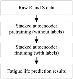
In this paper, the fatigue life prediction task is considered as a regression problem. The network takes the $R$ and $S$ as inputs and takes the $N$ as output. In the training procedure, the network analyzes the history data and learns the relationship among $R$, $S$, and $N$. In the testing time, we use the trained model to predict fatigue life, even the $R$ and $S$ never seen by model. The overall scheme of the presented method is shown in Fig. 2.

As shown in Fig. 2, the stacked autoencoder was greedy layer-wise trained without labels at first, then supervised learning was performed to fine-tune the relationship among $R$, $S$, and $N$. After the training, the model can predict the fatigue life using input.

In traditional research, the S-N curve was acquired under certain roughness, so there will be necessary to calculate a lot of S-N curves which is inconvenient. But in this paper, we build the relationship between $R$, $S$, and $N$ on one stage. The model not only learned the effect of $S$ on $N$, but also analyze the effect of $R$ on $N$.

The collected sets of experiment data are used to train the model where the roughness and stress are the raw signals passed to autoencoder. The mean value of fatigue life serves as the validation data because the fatigue life is not a constant in the experiment.

Fig. 1The structure of deep autoencoder

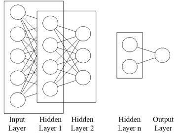
Fig. 2The overall procedure of presented method

3. Experimental setup

The material researched is medium-carbon, and its material property was shown in Table 1. The geometry of the specimen is shown in Fig. 3. To investigate the impact of difference surface roughness on fatigue life of specimen, specimens were machined into three groups.

As shown in Fig. 3, the finest part located in the middle of the specimen is 3.5 mm in diameter, where the stress is also the largest of the specimen. The stress data calculated by the applied load.

Fig. 3Fatigue specimen geometry (dimensions in mm)

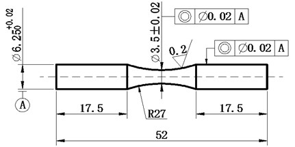
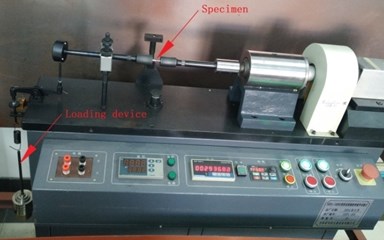
Fig. 4 shows the experimental setup. It consists of a fixed end, a specimen clamping device, a support device, a loading device, and a fatigue life statistical device. It can be seen from Fig. 4, the magnitude of the load is determined by the weight of the loading device, so the stress loaded on the specimen is calculated based on the counterweight.

The fatigue tests were performed 75 times with three different kinds of roughness ($R=$ 0.4, 0.8, and 1.6 μm) and five stress levels (550, 500, 450, 400, and 380 MPa). The same roughness and the stress test were performed 5 times. In addition, 6 sets of 420 MPa level stress were performed under three roughness conditions to test the model's performance.

Fig. 4The testing apparatus

4. Result

The specimens were tested five times under each experimental condition. A total of 75 experiments were conducted, and 75 sets of useful data were collected. And then use the 75 sets of data to train the deep learning model which was previously designed. After the model training is completed, we predict the life of the three different roughness specimens under different stress levels by using the model.

Fig. 5The S-N curves and fatigue life mean distribution

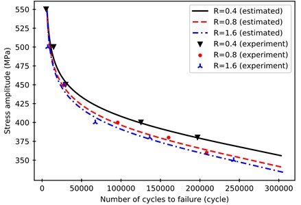
Fig. 5 show the difference between the difference between the true life and the mean value. It can be seen from Fig. 5 that the model can predict the life of the medium carbon steel well and the predicted life is close to the mean of the life of the experiment. This shows that the model also filters out some noise to some extend and finds out the relationship between roughness, stress, and life.

In order to further evaluate the effectiveness of the model, compare the results from the model in this paper with the predicted results based on the Tanaka-Mura model, Fig. 6 is the S-N curve based on the Tanaka-Mura theory. Compared with Fig. 5, the basic trend of the two is similar, but the prediction value of the model in this paper is closer to the mean value of the real life of the specimen [10]. Based on the Tanaka-Mura theory, the S-N curves of 0.4 and 0.8 roughness are very close (the formulas used comes from the paper of Li C. et al. [1]) and little apart from the experimental data point.

There are significant differences between the S-N curves based on different theory. It can be seen in Fig. 6 that the Tanaka-Mura model fit the real data poorly especially the curve of $R=$ 0.4, although the parameters calculated by the raw data. On the contrary, the neural network model builds the relationship between $R$, $S$, and $N$ with a smaller gap than Tanaka-Mura model. Furthermore, the method presented in this paper almost need no prior knowledge.

It can be concluded that the presented model is suitable than Tanaka-Mura model to calculate $N$. As shown in Fig. 5, the curves of $R=$ 0.8 and 1.6 μm are very close and have a big gap with $R=$ 0.4 μm, which can be explained that $R$ has a significant influence on the initiation of a crack. When the $R$ is very small, the crack initiation life $N_i$ mainly influenced by the $R$. With the increasing of $R$, the $N_i$ tends to a constant value and crack propagation life $N_p$ is the primary factor of fatigue life difference [11]. Meanwhile, the fatigue life is mainly affected by the $S$ at the high stress (great than the yield strength). It is reasonable for the steel because the specimen tends to break due to the static strength damage.

To evaluate the presented model is more accurate than Tanaka-Mura, a set of data under 420 MPa stress level was used to test two models. From the result (Table 2) of testing, it can be seen that the presented method is more accurate. The result also can prove the above explanations about the roughness’s impact on fatigue life.

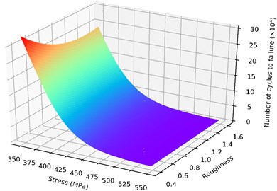
The model established in this paper not only predicts the life of the specimen under the surface roughness used in the experiment, but also predicts the fatigue life of the material with different surface roughness at a certain stress level. Fig. 7 is the fatigue life prediction of carbon steel for the different surface roughness and stress through the model.

Fig. 7 shows the relationship between $R$, $S$ and $N$. Medium-carbon fatigue life is largely affected by stress: as the stress increases, the fatigue life decreased rapidly. In addition, roughness is also a key factor in fatigue life while there is low stress and $R=$ 0.4 and 0.8 μm. On the other hand, the above conclusion about the effects of $R$ and $N$ on $N_i$ and $N_p$ are verified here.

Fig. 6The S-N curves based on Tanaka-Mura theory

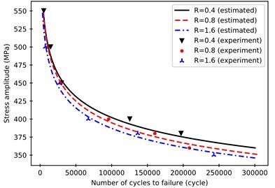
Fig. 7The prediction of medium-carbon life with different roughness and stress

5. Conclusions

In this paper, the fatigue life data of carbon steel was modeled using the deep autoencoder. In order to verify the effectiveness of the deep learning method, 75 sets of experimental data were used to train the model. Using the mean value of the specimen (15 groups) to test the model, and in the end, compared with other theoretical predictions. The life expectancy obtained by the learning model is closer to the mean value of the life of the specimen, which indicates that the model in this paper predicts better results. If we can increase the amount of experimental data, we can expect the model to bring more accurate predictions. In addition, we explore the effects of stress and roughness on crack initiation life and crack propagation life.