Abstract
To reduce the adverse effect of incorrect parameters for the traditional iterative tunable Q-factor wavelet transform, this paper proposes an iterative tunable Q-factor wavelet transform method for fault feature extraction. Firstly, before decomposing the bearing vibration signal by an iterative tunable Q-factor wavelet transform, the initial values of 3 basic factors should be set: the quality factor Q, redundancy r and the number of decomposition level . Secondly, the kurtosis of a high resonance component, which is the result of an iterative tunable Q-factor wavelet transform, is calculated through multistep iteration until it meets the iteration stop condition. Finally, the envelope spectrum of the final low resonance component is calculated, and the type of bearing fault can be recognized according to the frequency of extreme points. The results show that this method can effectively suppress noise and in-band interference and avoid fault identification inaccuracies caused by improper parameters and can also identify the fault feature frequency more clearly.
1. Introduction
In recent years, on the basis of the traditional Fourier transform, wavelet denoising has been widely used in practice by many scholars because of its low entropy, multi-resolution, correlation and flexibility. Chen et al. [1] proposed a data driven threshold strategy for different wavelet coefficients. Selesnick [2] first proposed a Tunable Q-factor Wavelet Transform (TQWT) in 2011. Li Xing [3] applied the genetic algorithm to the Q-factor optimisation with the iterative tunable Q-factor wavelet transform method to avoid the blindness of the Q-factor selection.
Different from the previous fixed Q value algorithm, the algorithm proposed in this paper separates the high and low resonance component layer by layer by iterating the size of the Q-factor step by step and eliminates the noise signal from the low resonance component. Then, the spectral kurtosis of the decomposed high resonance component will decide whether the low resonance component will be decomposed continuously. Finally, the envelope spectrum is obtained from the low resonance component after the cycle termination, and the type of fault is judged according to the frequency of the extreme point. The results show that the method can effectively suppress the noise components in the low frequency component. Compared with the traditional envelope spectrum method, this method can effectively extract the fault characteristic frequency and detect the early faults of bearings.
2. Iterative tunable Q-factor wavelet transform
The resonance property of signal is defined by the Q-factor. The larger the Q-factor is, the better the frequency aggregation of signals and the higher the resonance property are, the smaller the Q-factor is, the better the time aggregation of signals and the lower the resonance property are. The basic idea of the algorithm is to decompose a noisy and interfered signal with two different wavelet basis functions.
The wavelet basis function with high Q-factor is used to represent the components with strong oscillation in the signal. Low Q-factor is used to represent the components with weak oscillation.
The iterative tunable Q-factor wavelet transform method combines the signal center frequency and frequency bandwidth synthetically with the signal resonance attribute. It can effectively separate the central frequency and the overlapping of the central frequency bands and has different signal components with different Q-factors.
2.1. The tunable Q-factor wavelet transform (TQWT)
The tunable Q-factor wavelet transform is a flexible discrete wavelet transform. The is defined directly in the frequency domain, in which is the central frequency of the signal and is the bandwidth. According to the different characteristics of the signal oscillation, the Q-factors of the wavelet transform can be adjusted flexibly. Similarly, to other kinds of wavelet transform, TQWT is also based on multichannel filter, and its filtering principle is shown in Fig. 1. A series of two channel filter banks are used to decompose the low frequency band of the signal through iteration. The wavelet factor of the sub signal is expressed by (). LPS and HPS are the low-pass scale and the high-pass scale, and are the low-pass scale parameter and the high-pass scale parameter, which represent the increase or decrease of the sampling frequency. That is to say, the next ordered sampling frequency is (low-pass frequency band) or (high-pass frequency band) times before, as shown in Fig. 1. In order to reconstruct the signal better, the filter bank must be strictly sampled, and the value of and must strictly satisfy the condition , , . The base –2 fast Fourier transform is used here to improve the computational efficiency.
Fig. 1Schematic diagram of the tunable Q-factor wavelet transform filter
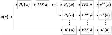
a) The principle of TQWT decomposition filter
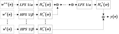
b) The principle of the TQWT synthetic filter
The definition of the frequency response function and of the high and the low pass filter are as follows:
where , is a Debbie Keyes (DB) frequency response. In these parameters, the high-pass scale parameter is directly related to the Q-factor: . The relationship between the low pass scale parameter and the redundancy is . When is kept constant, the redundancy increases, the degree of overlap between the frequency response of the wavelet will increase. So, the large is, the larger the decomposition level will be required to cover the same frequency range. Because the signal cannot be decomposed infinitely, the maximum amount of decomposition is determined by the Eq. (3):
where represents the largest integer less than and represents the length of the signal. Therefore, if the quality factor , the redundancy , and the decomposition level are determined, then a definite adjustable Q-factor wavelet transform can be defined.
2.2. Separation of high resonance and low resonance components
The method of iterative tunable Q-factor wavelet transform uses morphological component analysis (MCA) to separate the components in the signal according to the oscillation characteristics and establish the best representation of the high resonance component and the low resonance component.
The signal through the adjustable Q-factor wavelet transform can get 2 kinds of wavelet basis function library and with quality factors and . The signal to be decomposed can be expressed as follows:
In the formula, and are wavelet transform coefficients. and are the low resonance component and the high resonance component of the signal to be decomposed, and is called the residual component of the signal to be decomposed, which cannot be expressed by or .
If there are many minimum elements in the coefficient matrix and , and the residual component is very small, then Eq. (4) is a sparse representation of the signal to be decomposed. The purpose of MCA is to separate source signals from signals to be decomposed. In order to achieve effective separation of the high resonance component and the low resonance component, the objective function of morphological component analysis can be expressed as:
The weight coefficients and in the Eq. (5) determine the optimal coefficient and , and determine the energy of the high resonance component and the low resonance component in the final decomposition.
Eq. (5) considers the sparsity of the wavelet transform coefficient , and the size of the residual component in the Eq. (4). The smaller the values of the objective function, the sparser the decomposition is.
The optimal coefficient and are obtained by using the Split Augmented Lagrangian Shrinkage Algorithm (SALSA) [4]. The process of sparse decomposition is to find and when the function reaches a minimum. The estimated values of the high resonance component and the low resonance component are expressed as:
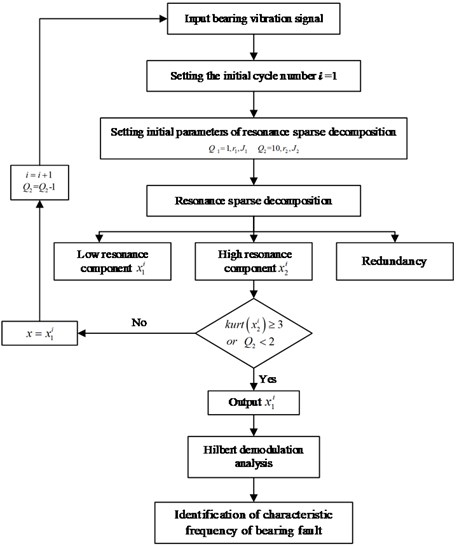
The tunable Q-factor wavelet transform can decompose input signals into high and low resonance components. The main components of the high resonance component are interference signal and noise. The spectral kurtosis should be less than 3. The main component of the low resonance component is the transient impact signal, and its spectral kurtosis should be more than 3. Therefore, when the bearing fault vibration signal is decomposed by iterative tunable Q-factor wavelet transform, the spectral kurtosis index can be used to determine whether there are still noise and interference signal residues in the low resonance component after decomposition, and whether further decomposition of different Q-factor is needed. If the spectral kurtosis of the high resonance component is greater than 3 after several decompositions, it is proved that some of the transient impact components have been decomposed into the high resonance component. This means that there is no residual interference signal and noise in the low resonance component at this time. So, in every iteration, the spectral kurtosis of the high resonance component will be calculated. If its value is less than 3, the low resonance component obtained from this cycle will be used as the input signal of the next cycle, and the iteration process will continue. Otherwise, the iteration will terminate, and the output is the low resonance component of the iterations. The iterative tunable Q-factor wavelet transform flow chart is shown in Fig. 2.
Fig. 2Principle flow chart of the rolling bearing early fault diagnosis based on the iterative tunable Q-factor wavelet transform
3. Experimental verification
The accelerometer is installed in the vertical and horizontal position of the bearing. The experiment used the acceleration sensor of 100 K. In order to verify the effectiveness of the method, the inner and outer ring fault experiments of the rolling bearing were carried out. The NTN6204 type rolling bearing was used in the experiment to simulate the inner and outer ring faults. Two grooves both with a width of 0.7 mm and the depth of 0.25 mm were cut by laser on the inner ring and outer ring of the bearing. The vibration signal was collected by the acceleration sensor. The sampling frequency was 100 kHz, the number of sampling points was 32 768, and the rotation speed of the rolling bearing 900 r/min. Fig. 3 shows the time domain waveform of the bearing in normal state. According to the calculation formula in the literature [5], the frequency of fault features of the outer ring and inner ring is 59.76 Hz and 100.97 Hz. In order to simulate the vibration signal at the initial stage of the bearing, Gauss white noise with signal to noise ratio was added. The setting parameter value of the iterative tunable Q-factor wavelet transform is shown in Table 1.
Fig. 3Time domain diagram of bearing under normal condition
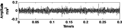
Table 1Parameters of the iterative tunable Q-factor wavelet transform
Signal type | Filter Library | Quality factor | Redundancy factor | Decomposition level | Weight coefficient |
Fault signal of bearing outer ring | High resonance filter Library | 9 | 5 | 1.1 | |
Low resonance filter Library | 1 | 5 | 1 | ||
Fault signal of bearing inner ring | High resonance filter Library | 13 | 5 | 0.1 | |
Low resonance filter Library | 1 | 5 | 0.15 |
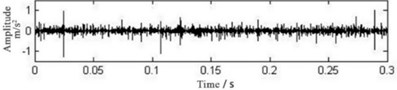
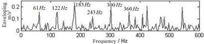
The original signal diagram of the rolling bearing outer ring fault is shown in Fig. 4. Firstly, the iterative tunable Q-factor wavelet transform method proposed in this paper is used to denoise. When the iteration is carried out once, the termination condition is satisfied. In this case, the spectral kurtosis of the high resonance component is 16.3349. Since the noise is more concentrated in the high frequency component, the information in the low resonance component preserves a large number of vibration shock signals after the iteration. The time-domain waveform of the low resonance component is shown in Fig. 5, it can be seen that the time-domain waveform noise is obviously reduced. After using the Hilbert envelope demodulation for the low resonance component, the characteristic frequency of 61 Hz and its frequency doubling components are obtained, and the envelope spectrum is shown in Fig. 5.
Fig. 4Time-domain waveform diagram of fault original signal of bearing outer ring
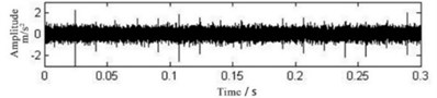
Fig. 5Time-domain waveform diagram and envelope spectrum of the low resonance component with the iterative tunable Q-factor wavelet transform
The time-domain waveform of the fault vibration signal of the rolling bearing inner ring is shown in Fig. 6. The impact component is not obvious enough to obtain. Additionally, the impact component needs to be further extracted from the signal. After performing the iterative tunable Q-factor wavelet transform twice, the spectral kurtosis of the high resonance component is 2.7456 and 3.0482 respectively. The time-domain waveform of the low resonant component is shown in Fig. 7, and the envelope spectrum of the low resonance component is shown in Fig. 7 in which the fault characteristic frequency at 100 Hz is obvious. The result shows that this method can effectively diagnose the rolling bearing failure.
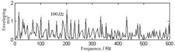
As a comparison, the traditional signal iterative tunable Q-factor wavelet transform method is carried out with the same parameters through decomposing and envelope demodulation for the fault signal of bearing inner ring. The result of the envelope spectrum is shown in Fig. 8. The fault characteristic frequency is drowned in the noise and the types of the fault cannot be identified directly. From the comparison and analysis above, it can be seen that the method in this paper is better than the traditional iterative tunable Q-factor wavelet transform method for bearing fault diagnosis.
Fig. 6Time-domain waveform diagram of fault original signal of bearing inner ring
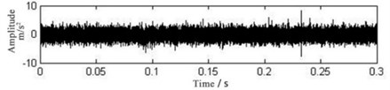
Fig. 7Time-domain waveform diagram Envelope spectrum of the low resonance component with iterative tunable Q-factor wavelet transform

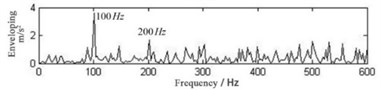
Fig. 8Envelope spectrum of fault signal of bearing inner ring by traditional tunable Q-factor wavelet transform
4. Conclusions
This study has proposed a method that consists in adjusting the value of the high Q-factor and then filtering step by step. It thus avoids the problems of incomplete filtering and inaccurate identifying by using fixed double Q value for the single iterative tunable Q-factor wavelet transform. The algorithm simulation and application example show that this method can effectively remove the strong noise and interference in the signal and extract the transient impact components in the bearing fault signal.
References
-
Chen Y. M., Zi Y. Y., Cao H. R., et al. A data-driven threshold for wavelet sliding window denoising in mechanical fault detection. Science China Technological Sciences, Vol. 57, Issue 3, 2014, p. 589-597.
-
Selesnick I. W. Wavelet transform with tunable Q-factor. IEEE Transactions on Signal Processing, Vol. 59, Issue 8, 2011, p. 3560-3575.
-
Li Xing, Yu De-Jie, Zhang D. C. Fault diagnosis of rolling bearings based on the iterative tunable Q-factor wavelet transform with optimal Q-Factor. Journal of Vibration Engineering, 2015.
-
Afonso M. V., Bioucasdias J. M., Figueiredo M. A. Fast image recovery using variable splitting and constrained optimization. IEEE Transactions on Image Processing, Vol. 19, Issue 9, 2010, p. 2345-2356.
-
Jiang Jingsheng Research on Fault Feature Extraction and Recognition Based on Local Tangent Space Alignment Algorithm. Beijing University of Chemical Technology, 2017.
About this article

This research was supported by The National Key Research and Development Program of China (2018YFC0809004).
