On a method of applied symbolic dynamics for investigation of dynamical systems

Ampilova, Natalia; Soloviev, Igor

doi:10.21595/vp.2019.20698

Vibroengineering Procedia

Browse Procedia

Published: 25 June 2019

Check for updates

On a method of applied symbolic dynamics for investigation of dynamical systems

Natalia Ampilova¹

Igor Soloviev²

^{1, 2}St. Petersburg State University, St. Petersburg, Russia

Corresponding Author:

Igor Soloviev

Cite the article Download PDF

Downloads 1421

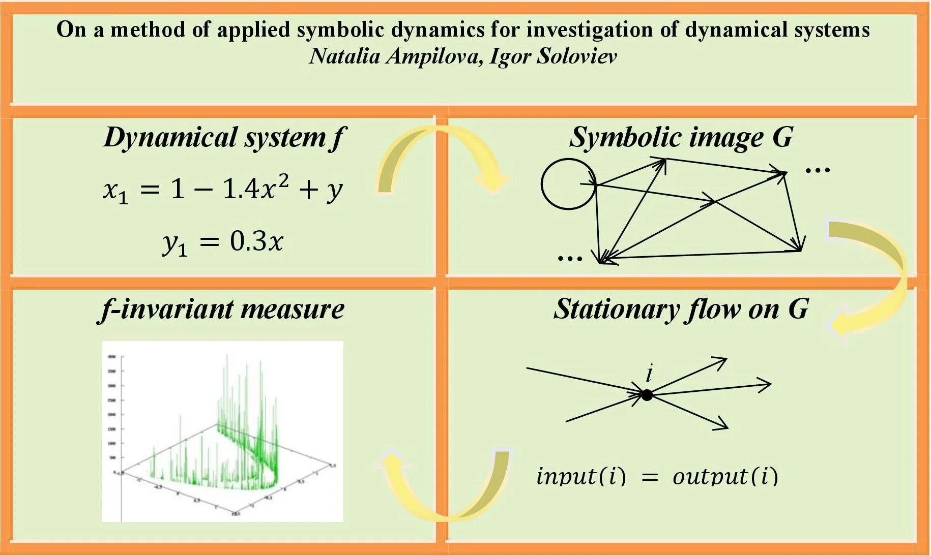
Abstract

We consider a method of applied symbolic dynamics which may be used to obtain wide spectrum of characteristics of complex dynamical systems: approximation of invariant sets, estimation of topological entropy and approximation of invariant measures. The method has received wide acceptance in studying complex dynamical systems. The main idea of the method is to describe the system behaviour approximately by means of an oriented graph (called symbolic image). Such a graph is a representation of symbolic dynamical system which is more appropriately known as topological Markov chain. There exists a correspondence between trajectories of a given system and paths on the graph, which allows us to design algorithms for estimation of topological entropy, approximate invariant measures of a given system by using stationary flows on the graph and calculate corresponding metric entropies. These values characterize complex behaviour of dynamical systems such as the existence of trajectories with large periods and chaotic regimes. The results of experiments are given for systems with chaotic dynamics.

On a method of applied symbolic dynamics for investigation of dynamical systems

Highlights

Symbolic dynamics allows a coding smooth dynamical systems.
Reasonable coding results in an acceptable correspondence between a given system and the coded one.
Symbolic image is the coding by using oriented graph such that ε-trajectories of a given system are represented by paths on the graph.
Invariant measures of a given system are approximated by stationary flows on the graph and topological entropy of the symbolic image is an upper bound for the given system entropy.

1. Introduction

Symbolic dynamical systems form an important class of dynamical systems. They are defined on the space of infinite symbol sequences which are constructed as words over a finite alphabet. On such a space one may consider shift operator that shifts a sequence one symbol left. These systems are often used for the coding smooth dynamical systems. The coding means that we consider a finite partition of a phase space and assign a symbol from a finite alphabet to each element of the partition. Then a trajectory may be written (coded) as a symbol sequence in accordance with the transition of a trajectory from one partition element to another, being one step along the trajectory corresponds to one step in symbol sequence, i.e. the action of shift map. The coding describes the order in which the points of a trajectory visit elements of the partition.

The methods implementing ideas of symbolic dynamics are said to be applied symbolic methods. The work of J. Hadamar [1] published in 1898 is likely the first example of the application of symbolic dynamics. The author used trajectory coding for description of global behavior of geodesics on the surfaces with negative curvature. H. Morse and G. Hedlung [2, 3], and R. Bowen [4] contributed significantly to the progress of the method. V. Alekseev [5] applied it for celestial mechanics problems. To study global structure of dynamical systems C. Hsu elaborated “cell-to-cell mapping” method [6]. He considered cells of a given partition and their images under the action of a system. Two variants of such mapping were proposed, but symbolic dynamics was not used. M. Delnitz, A. Hohmann and O. Junge [7, 8] considered set-oriented methods that use graph for representation of the dynamics of a system and the subdivision technics to refine the initial covering and obtain more detailed information about the system behaviour. Symbol sequences were not used.

Of particular interest is the application of symbol sequences to study chaotic attractors in discrete discontinuous systems which are models of inverter systems [9], and in periodic nonautonomous systems [10, 11], where the authors considered stroboscopic map and analysed its behaviour by using symbolic dynamics.

The method of symbolic image in which the transitions of a trajectory between partition elements are represented by an oriented graph was proposed by G. Osipenko [12]. This approach combines C. Hsu’s idea and symbolic dynamics. The obtained graph is the topological Markov chain defined by its adjacency matrix, and symbol sequences correspond to paths on the graph. This method was successfully applied to approximation of invariant sets and Morse spectrum [13].

In this work we propose the approach to the investigation of dynamical systems which is based on ideas of the symbolic image method and allows us to elaborate algorithms for an approximation of invariant measures of dynamical systems and estimation of such important characteristics as topological and metric entropy.

Any invariant measure of the system generates a stationary flow on the graph of symbolic image. To construct such a flow, we designed and implemented algorithms which are based on finding simple cycles (the algorithm was implemented for 3 variants of assigning weight to a cycle), and the balance method. It is significant that by constructing stationary flows by different ways we obtain an interval for metric entropies, being the method of simple cycles gives minimal value for metric entropy and the balance method gives maximal one. Topological entropy calculated by adjacency matrix of symbolic image turns out to be more than maximal metric entropy. To illustrate our approach, we give numerical results for two chaotic maps.

2. Symbolic dynamics

2.1. Space of sequences

Symbolic dynamical systems are defined on the space of symbol sequences and may be models for smooth dynamical systems or used for their coding.

For a given natural number $m \geq 2$ consider the space of bi-infinite sequences of the form:

1

Ω_{m} = \{ω = (\dots, ω_{- 1}, ω_{0}, ω_{1}, \dots), ω_{i} \in \{0,1, \dots, m - 1\}, i \in Z\} .

By the same way one may consider the space of infinite sequences:

2

Ω_{m}^{R} = \{ω = (ω_{0}, ω_{1}, \dots), ω_{i} \in \{0,1, \dots, m - 1\}, i \in N\} .

For the space defined by Eq. (1) shift map $σ$ is introduced as:

σ : Ω_{m} \to Ω_{m}, σ (ω) = ω^{'} = (\dots ω_{0}^{'}, ω_{1}^{'}, \dots), ω_{n}^{'} = ω_{n + 1},

and for Eq. (2) shift map may be defined analogously. The restriction of shift map $σ$ on any closed invariant set $Ω_{s}$ of the space of sequences is said to be symbolic dynamical system.

2.2. Topological Markov chain

Topological Markov chains form the class of symbolic dynamical systems which is defined as follows. Consider space $Ω_{m}$ and ${0, 1}$ -matrix $A = \{a_{i j}\}$ , $i, j \in \{0, m - 1\} .$

Now construct the space of sequences defined by $A$ in the following manner:

3

Ω_{A} = \{ω \in Ω_{m}, a_{ω_{n} ω_{n + 1}} = 1\} .

In other words, according to Eq. (3) elements of $A$ mark transitions in sequences of symbols, and we consider the sequences in which there are only admissible transitions. It is easy to note that $Ω_{A}$ is $σ$ -invariant. The restriction of $σ$ on $Ω_{A}$ is said to be topological Markov chain defined by matrix $A$ . This construction is widely used in application because it may be represented by the oriented graph with adjacency matrix $A$ .

2.3. Coding of smooth systems

Consider a dynamical system generated by a homeomorphism $f$ defined on a set $M$ and a finite partition ${{M}_{i}}$ , $i = 1, \dots, n$ . It is easy to understand that:

4

x \in \cap_{k = 0}^{n - 1} f^{- 1} (M_{i_{k}}) \Rightarrow f^{k} (x) \in M_{i_{k} .}

The intersections of such a kind may contain more than one point, and it means that several trajectories will be coded by one symbolic sequence.

If we place the restriction that the intersection in Eq. (4) consists of one point, one may consider a continuous and onto map $h$ (a factor map) between the symbolic dynamical system and the initial one, such that $h \circ σ = f \circ h$ . In this case dynamical system $(M, f)$ is said to be factor of dynamical system $(Ω_{s}, σ)$ , and there is a semi-conjunction between the systems. If the systems considered are conjugate, we have exact coding, as for the Smale horseshoe (when system trajectories are coded by binary sequences), and hyperbolic automorphism of torus.

The connection between a smooth system and its symbolic representation defines the estimation of topological entropy of the first one. If $f$ is factor of $σ$ then topological entropy $f$ less or equal topological entropy $σ .$ Hence in this case the transition to a symbolic dynamical system allows us to obtain an upper bound for the entropy of the given system. Conjugated systems have the same entropies. Unfortunately, for arbitrary system we have no prior knowledge of the type of connection between the given and symbolic systems. Note that the using topological Markov chain makes it possible to obtain upper bound for topological entropy by easier way.

3. Symbolic image of a dynamical system

For a discrete dynamical system defined by a homeomorphism $f$ and the given partition ${{M}_{i}}$ the corresponding symbolic dynamical system is constructed as follows. For each $M_{i}$ we consider its image $f (M_{i}$ ) and find all $M_{j}$ such that $f (M_{i}) \cap M_{j} \neq \emptyset .$ Let $G$ be a directed graph in which vertices ${i}$ correspond to cells ${{M}_{i}}$ , and there is edge $i \to j$ iff $f (M_{i}) \cap M_{j} \neq \emptyset .$ Then $G$ is said to be the symbolic image of $f$ with respect to the partition ${{M}_{i}}$ .

For symbolic image the following parameters are defined: $d$ – maximal diameter of ${{M}_{i}}$ , $q$ – maximal diameter of $f (M_{i}$ ), $r$ – low bound, the smallest distance between $f (M_{i}$ ) and $M_{k}$ such that $f (M_{i}) \cap M_{j} = \emptyset .$

Let $ε > 0$ be given. A bi-infinite sequence ${x_{k}, k \in Z}$ is called $ε$ -trajectory (or pseudo-trajectory) of $f$ if for any $k$ we have $d i s t (f (x_{k}), x_{k + 1}) < ε$ . A pseudo-trajectory is called $p$ -periodic if $x_{k} = x_{k + p}$ for each $k$ . Note that in calculation we operate with an approximation of real trajectories with some small $ε$ .

In what follows we assume that a path on a graph of symbolic image is written as a sequence of vertices. There is a correspondence between trajectories of initial system and paths on the graph of symbolic image, such that a set of $ε$ -trajectories corresponds to one path on the graph, and we will not obtain exact coding. The main idea of the symbolic image method is to construct a sequence of partitions for $d \to 0$ , the sequence of corresponding them symbolic images and a special mapping between paths of symbolic images. It has been proved [12] that in the limit we obtain the correspondence “one trajectory-one path”.

4. The estimation of the complexity of dynamical systems

4.1. Topological entropy

There are several methods to define topological entropy of a dynamical system, for example through minimal coverings or separated sets [14]. For some systems it coincides with the growth rate of periodic orbits and may be calculated easily (linear extending maps, hyperbolic automorphism of torus). But for the most part of systems direct calculations are difficult and we should use methods of estimations. S. Newhouse and T. Pignataro [15] proposed to estimate the topological entropy of a smooth dynamical system by calculating the logarithmic growth rates of suitably chosen curves in the system (entropy on the curve length). The method may be successfully applied for studying the complex system having strange attractors. Topological entropy with relative ease may be obtained for topological Markov chain as the module of maximal eigenvalue of the adjacency matrix for the correspondent graph. It was shown in [12] that the entropy of a given dynamical system not greater than the entropy of symbolic image, in other words symbolic image allows us to obtain an upper estimation.

4.2. Metric entropy

Another approach to the obtaining characteristics of dynamics is statistical description of orbit behavior. For this purpose, measure-preserving transforms are considered. A mapping $f : X \to X$ is said to be measure $μ$ preserving (or $μ$ is invariant measure for $f$ ), if for any measurable set $A$ the set $f^{- 1} (A)$ is measurable and $μ (f^{- 1} (A)) = μ (A) .$ For any invariant measure $μ$ one may calculate metric entropy of the map $f,$ and according to variational principle, topological entropy is supremum of metric entropies. One can say that metric entropy accounts for average complexity of a system, whereas topological entropy measures its maximal dynamical complexity.

In practical applications it is of value to construct an approximation to an invariant measure for a dynamical system, and calculate metric entropy by this measure to obtain lower bound for topological one. The symbolic image method may be effectively applied to solve this problem.

Consider an invariant measure $μ$ for a dynamical system $f$ . Then we assign to an edge $(i \to j)$ value $μ (f (M_{i}) \cap M_{j})$ , from which the relation $\sum_{j} μ (f (M_{i}) \cap M_{j}) = μ (f (M_{i}) = μ (M_{i})$ follows. By the same way we assign an edge $(j \to i)$ value $μ (f^{- 1}$ ( $M_{i}) \cap M_{j})$ and obtain:

\sum_{j} μ (f^{- 1} (M_{i}) \cap M_{j}) = μ (f^{- 1} (M_{i})) = μ (M_{i}),

so the constructed flow on the symbolic image graph is stationary, i.e. for any vertex the sum of weights of incoming edges is equal to the sum of weights of outcoming ones. One may say that an invariant measure of a dynamical system generates a stationary flow on symbolic image. Usually the normed flow is considered.

It is known that the set of all invariant measures for a system $f$ is closed convex set in weak topology [14], and the convergence $μ_{n} \to μ$ in this topology means that for any continuous function $φ : M \to R$ we have $\int φ d μ_{n} \to \int φ d μ$ .

The structure of the set of flows and the connection between the set $D (f)$ of $f$ – invariant measures and the set $D (G)$ of stationary flows on symbolic image $G$ was formulated and proved in [16] as the following statement.

Theorem. For any neighborhood (in weak topology) $U$ of the set $D (f)$ there is a positive number $d_{0}$ , such that for any partition ${M_{i}}$ with maximal diameter $d < d_{0}$ and any stationary flow ${m (M_{i}) = m_{i}}$ on the symbolic image $G$ constructed in accordance with this partition the measure $μ_{1} (A) = \sum_{i} m_{i} v (A \cap M_{i}) / v (M_{i})$ , where $v$ is Lebesgue measure, lies in $U$ . $□$

Hence any measure calculated by a stationary flow on a symbolic image (which is density distribution for a measure of a given system) approximates an invariant measure of the initial system if we use the partition with the diameter small enough. Moreover, this theorem guarantees that set $D (G)$ approximates set $D (f)$ . This fact is the substantiation for numerical experiments.

In our investigations we used two methods for the construction of stationary flow on the symbolic image: 1) assigning values of edges of simple cycles, being weights for cycles were chosen by 3 different ways; 2) assigning values to all edges and applying balance method to obtain a stationary flow. The convergence of balance method was proved by L. Bregman in [17]. In [18] a lower bound of topological entropy for delay map and double logistic map was obtained. The metric entropy of the obtained stationary flow was calculated by the formula for topological Markov chain by Markov’s measure [14]. If a stationary flow on the graph is given by a vector $\{m_{i}\}$ (measures of vertices) and a transition matrix $P = {m_{i j}}$ and $\sum_{i, j} m_{i j} =$ 1, then metric entropy $h_{m}$ by this measure may be calculated as follows:

5

h_{m} = \sum_{i \in V} m_{i} \log m_{i} - \sum_{(i \to j) \in E} m_{i j} \log m_{i j},

where $G = (V, E)$ , and $V$ is the set of vertices and $E$ is the set of edges.

5. Examples

5.1. Henon map

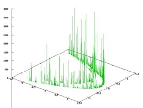
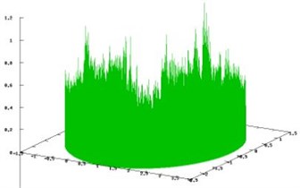
Consider the map $x_{1} = 1 - a x^{2} + y$ , $y_{1} = b x$ , where $a =$ 1.4, $b =$ 0.3, square $B =$ [–10, 10]×[–10, 10] and the initial partition consisting from 9 cells. On each step every cell is subdivided in 4 cells. After 6 iterations the number of vertices was 231. Values of metric entropy for 3 variants of the method of simple cycles are 0.551141, 0.656916, 0.685731. Metric entropy calculated by the measure constructed by balance method is equal to 1.384079.

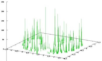
Logarithm of maximal eigenvalue of the adjacency matrix for $G$ (upper bound for topological entropy) is 1.386763. On Fig. 1 densities of invariant measures on the invariant set are shown: the method of simple cycles (Fig. 1(a)); balance method (Fig. 1(b)).

Fig. 1Densities of invariant measures constructed for the Henon map by the method of simple cycles (weights of all cycles are the same) and balance method

Densities of invariant measures constructed for the Henon map by the method of simple cycles (weights of all cycles are the same) and balance method

a)

b)

5.2. Ikeda map

Consider the map:

x_{1} = d - C_{2} (x \cos τ (x, y) - y \sin τ (x, y)), y_{1} = C_{2} (x \sin τ (x, y) + y \cos τ (x, y)),

where $τ (x, y) = C_{1} - \frac{C_{3}}{1 + x^{2} + y^{2}}$ , $d =$ 2, $C_{1} =$ 0.4, $C_{2} =$ 0.9, $C_{3} =$ 6.

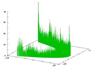
The calculations were performed on the area $B =$ [–10, 10]×[–10, 10]. After 10 step the graph contained 104799 vertices. Values of metric entropy for 3 variants of methods of simple cycles are 0.797314, 0.900477, 0.909025. Metric entropy calculated by the measure constructed by balance method is equal to 2.107914. Logarithm of maximal eigenvalue of the adjacency matrix for $G$ (upper bound for topological entropy) is 2.200624. On Fig. 2 the densities of invariant measures on the invariant set are shown for the method of simple cycles (weights of all cycles are the same) (Fig. 2(a)) and for balance method (Fig. 2(b)).

Fig. 2Densities of invariant measures constructed for the Ikeda map by the method of simple cycles (weights of all cycles are the same) and balance method

Densities of invariant measures constructed for the Ikeda map by the method of simple cycles (weights of all cycles are the same) and balance method

a)

b)

6. Conclusions

The method of symbolic image is used for coding smooth dynamical systems in such a way to describe the dynamics of a system by an oriented graph constructed in accordance with a given partition. By constructing a sequence of partitions using subdivision technique when diameters of partitions tend to zero we obtain the sequence of symbolic images, which gives a closer approximation to the system under study, and thereby a better correspondence between the initial system and its symbolic representation. An essential advantage of the method is that the symbolic image graph turns out to be topological Markov chain. Precisely because of this one may obtain an upper bound for topological entropy of the system as a maximal eigenvalue of the adjacency matrix of a symbolic image graph.

The proposed algorithms make it possible to approximate invariant measures of a given dynamical system by stationary flows on the graph of symbolic image. Depending on the method for the construction of a stationary flow one may obtain an interval for metric entropies, and in doing so for possible low bounds of topological entropy. Thus, practical application of the algorithms described permits to calculate characteristics that reveal the existence of complex and chaotic regimes in dynamical systems.

References

Hadamar J. Les surfaces a courbures opposees et leur ligues geodesiques. Journal De Mathematiques Pure Et Appliquees, Vol. 5, Issue 4, 1898, p. 27-73.

Search CrossRef
Morse H., Hedlung G. Symbolic dynamics I. American Journal of Mathematics, Vol. 60, Issue 4, 1938, p. 815-866.

Publisher
Morse H., Hedlung G. Symbolic dynamics II. American Journal of Mathematics, Vol. 62, Issue 1, 1940, p. 1-42.

Publisher
Bowen R. Symbolic Dynamics. American Mathematical Society Providence. R. I., Vol. 8, 1982.

Search CrossRef
Alekseev V. Symbolic Dynamics. 11 Mathematical School, Kiev, 1976.

Search CrossRef
Hsu C. S. Cell-To-Cell Mappling. a Method of Global Analysis for Nonlinear Systems. Springer, 1987, p. 64.

Search CrossRef
Dellnitz M., Hohmann A. A subdivision algorithm for the computation of unstable manifolds and global attractors. Numerische Mathematik, Vol. 75, 1997, p. 293-317.

Publisher
Dellnitz M., Junge O. Set Oriented Numerical Methods for Dynamical Systems. Handbook of Dynamical Systems II: Towards Applications. World Scientific, 2002, p. 221-264.

Publisher
Avrutin V., Schanz M. On the fully developed bandcount adding scenario. Nonlinearity, Vol. 21, 2008, p. 1077-1103.

Publisher
Avrutin V., Zhusubaliyev Z. T., Mosekilde E. Border collisions inside the stability domain of a fixed point. Physica D, Vol. 321, Issue 322, 2016, p. 1-15.

Publisher
Avrutin V., Zhusubaliyev Z. T., Mosekilde E. Cascades of alternating pitchfork and flip bifurcations in H-bridge inverters. Physica D, Vol. 345, 2017, p. 27-39.

Publisher
Osipenko G. Dynamical Systems, Graphs, and Algorithms. Lecture Notes in Mathematics, 1889. Tiergartenstrasse 17, Heidelberg, Germany, D-69121, 2007, p. 300.

Search CrossRef
Osipenko G. S., Romanovsky J. V., Ampilova N. B., Petrenko E. I. Computation of the Morse spectrum. Journal of Mathematical Sciences, Vol. 120, Issue 2, 2004, p. 1155-1166.

Publisher
Katok A., Hasselblatt B. Introduction to the Modern Theory of Dynamical Systems. Cambridge University Press, 1995.

Publisher
Newhouse S., Pignataro T. On the estimation of topological entropy. Journal of Statistical Physics, Vol. 72, 1993, p. 1331-1351.

Publisher
Osipenko G. Symbolic image and invariant measures of dynamical systems. Ergodic Theory and Dynamical Systems, Vol. 30, 2010, p. 1217-1237.

Publisher
Bregman L. M. The proof of the Sheleihovsky G. V. method for problems with transport restrictions. Journal of Computational Mathematics and Mathematical Physics, Vol. 7, Issue 1, 1967, p. 147-156, (in Russian).

Publisher
Ampilova N., Petrenko E. On application of balance method to approximation of invariant measures of a dynamical system. Differential Equations and Control Processes, Vol. 1, 2011, p. 72-84.

Search CrossRef

About this article

Received

30 March 2019

Accepted

23 April 2019

Published

25 June 2019

SUBJECTS

Chaos, nonlinear dynamics and applications

DOI

https://doi.org/10.21595/vp.2019.20698

Keywords

dynamical systems

applied symbolic dynamics

topological entropy

symbolic image

invariant measure

Acknowledgements

Authors wish to express their thanks to E. Petrenko for images.

This is an open access article distributed under the Creative Commons Attribution License, which permits unrestricted use, distribution, and reproduction in any medium, provided the original work is properly cited.

Previous article in issue Previous Next article in issue Next

Research article

2019 09 26

On application of dynamical system methods in biomedical engineering

Natalia Ampilova, Vladislav Sergeev, Igor Soloviev

Research article

2019 04 25

Topology optimization for vibrating structures with the BESO method

Christian Brecher, Guifeng Zhao, Marcel Fey

Research article

2019 03 15

A homogeneous high precision direct integration based on Chebyshev interpolation

Dongliang Chen, Lianfu Wang, Jindong Zhang

Research article

2018 06 30

Entropies in investigation of dynamical systems and their application to digital image analysis

Natalia Ampilova, Igor Soloviev

N. Ampilova and I. Soloviev, “On a method of applied symbolic dynamics for investigation of dynamical systems,” Vibroengineering PROCEDIA, Vol. 25, pp. 128–134, Jun. 2019, https://doi.org/10.21595/vp.2019.20698

Copy Extrica

Copied to clipboard!

TY  - JOUR
DO  - 10.21595/vp.2019.20698
UR  - https://doi.org/10.21595/vp.2019.20698
TI  - On a method of applied symbolic dynamics for investigation of dynamical systems
T2  - Vibroengineering PROCEDIA
AU  - Soloviev, Igor
AU  - Ampilova, Natalia
PY  - 2019
DA  - 2019/06/25
PB  - JVE International Ltd.
SP  - 128-134
VL  - 25
SN  - 2345-0533
SN  - 2538-8479
ER  - 

Copy Ris

Copied to clipboard!

@article{Soloviev_2019,
	doi = {10.21595/vp.2019.20698},
	url = {https://doi.org/10.21595/vp.2019.20698},
	year = 2019,
	month = {jun},
	publisher = {{JVE} International Ltd.},
	volume = {25},
	pages = {128--134},
	author = {Igor Soloviev and Natalia Ampilova},
	title = {On a method of applied symbolic dynamics for investigation of dynamical systems},
	journal = {Vibroengineering {PROCEDIA}}
}

Copy Bibtex

Copied to clipboard!

[1]I. Soloviev and N. Ampilova, “On a method of applied symbolic dynamics for investigation of dynamical systems,” Vibroengineering PROCEDIA, vol. 25, pp. 128–134, Jun. 2019, doi: 10.21595/vp.2019.20698.

Copy IEEE

Copied to clipboard!

Soloviev, Igor, and Natalia Ampilova. “On a Method of Applied Symbolic Dynamics for Investigation of Dynamical Systems.” Vibroengineering PROCEDIA 25 (June 25, 2019): 128–34. https://doi.org/10.21595/vp.2019.20698.

Copy Chicago

Copied to clipboard!

On a method of applied symbolic dynamics for investigation of dynamical systems

Abstract

Highlights

1. Introduction

2. Symbolic dynamics

2.1. Space of sequences

2.2. Topological Markov chain

2.3. Coding of smooth systems

3. Symbolic image of a dynamical system

4. The estimation of the complexity of dynamical systems

4.1. Topological entropy

4.2. Metric entropy

5. Examples

5.1. Henon map

5.2. Ikeda map

6. Conclusions

References

About this article

Related Articles