Abstract
The development of imaging has always been the top priority of modern medical advancement. There are also many methods for image processing in brain. 3D Slicer is an open source medical software that can reconstruct and visualize various medical image data in three dimensions. Three-dimensional reconstruction of blood vessels, hematomas, and nerve fiber tissue in brain can better assist doctors in planning operation and surgical implementation.
Highlights
- Introduced an open source free and efficient medical image processing platform.
- Three-dimensional reconstruction of Brain CT data.
- Three-dimensional reconstruction of cerebral nerve bundle.
1. Introduction
3D Slicer (hereinafter referred to as the Slicer) is a free and open source, highly extensible, medical image processing and visualization of medical image processing and analysis of application platform, which is originated in the 1998 Boston brigham and women’s hospital surgery plan laboratory and artificial intelligence laboratory at the Massachusetts institute of technology jointly launched a master’s thesis project. The aim is to develop an easy to use software analysis, and visualization. Basing on the experience of earlier research teams in the surgery planning laboratory of Massachusetts institute of technology and brigham and women’s hospital in Boston, David Gering first proposed the Slicer prototype in his master's thesis in 1999. Subsequently, Steve Pieper served as the chief architect of the Slicer, commercializing the Slicer development effort to meet the requirements for industrial-scale installation packages.
The development of Slicer has been the focus of the surgical planning lab led by Ron Kikinis since 1999. Nowadays, most of the development work of Slicer is completed by professional engineers, algorithm developers and scientists in the application field. Meanwhile, Isomics Company, Kitware Company and GE global research institute and other companies join in the development of Slicer. Meanwhile, the growing Slicer community also makes great contributions to its development. Slicer was originally conceived as a system for neurosurgical-guided therapy, visualization, and analysis. However, over the past few decades, slicer has become a comprehensive platform for both clinical and preclinical research applications, as well as for non-medical image analysis.
The development and maintenance of Slicer are mainly funded by the national institutes of health, at the same time, Slicer also benefited from its massive developer community. Recording to the report sent by various teams and individual users, the community proposes the solutions of problems and the development of new tools to continuously improve and expand the function of the Slicer.
The major features of Slicer are broad functionality, good scalability, platform independence, and unlimited software licensing, which are unmatched by other slicer-like commercial and open source software tools or workstations.
Because commercial impact workstations and image analysis tools are often not extended by end users, development models are not tool-oriented and may require specialized hardware, their use in projects requiring new image analysis methods is limited. At the same time, many of the commercial image workstations and image analysis tools currently available are often very expensive, and not all academic researchers can afford these systems. Compared with these commercial workstations, Slicer provides free research platforms for academic researchers and requires no special hardware devices. In addition, Slicer supports multiple operating systems, such as Windows, Mac OS X and Linux [1].
2. Modeling
2.1. CT modeling
Computerized tomography, which uses precise collimation of X-ray beams, gamma rays, ultrasound, etc., together with a highly sensitive detector to scan a section of the human body one by one, with fast scanning time and clear image And other characteristics, can be used for the examination of a variety of diseases.
2.2. DICOM file import
DICOM (Digital Imaging and Communications in Medicine) defines a medical image format that can be used for data exchange with quality meeting clinical needs.
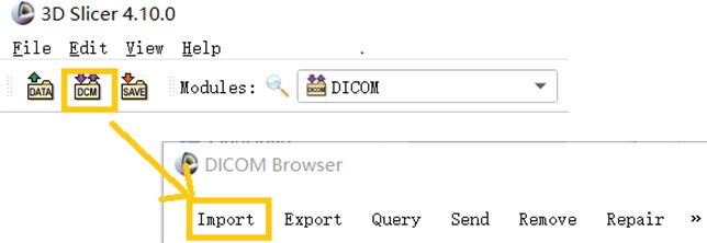
The DICOM data of a CT image is usually in serial form and consists of a sectional section image of a part of the human body. When using 3D Slicer to Import DICOM files, you can use the Import function in the DICOM module that comes with the software to Import CT images in the folder.
Fig. 1This image shows a partial screenshot of the software, showing the specifics of importing data
2.3. Mango
CT data often appears in the form of multiple folders after being carved. Direct import of 3D Slicer is simple and convenient, but the data is easy to be confused. Mango software can automatically distinguish the files that are mixed together according to the patient and the sequence. After opening the corresponding sequence, save it as a nii.gz file and drag it into the 3D Slicer software to apply it.
Fig. 2Mango software import operation
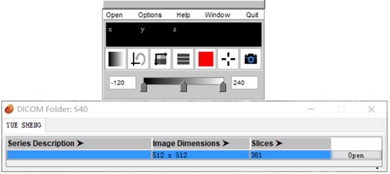
Mango software is a medical image processing software which developed by the University of Texas. Its unique file integration feature is especially outstanding. Mango is also very simple to use, just find the folder path and import it in the software [2].
2.4. Volumes module
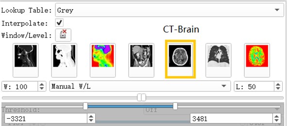
Volumes Module is the interface for adjusting Window, Level, Threshold, Color LUT and other parameters that control the display of volume image data in the scene [3].
After the data is imported successfully, you can see the horizontal axis of the CT image of the brain, the cross section of the sagittal axis and the direction of the coronal axis. It can be observed that the CT image just imported is lighter in gray and cannot clearly show the tissue and hematoma. This is caused by the CT value of the CT image being too large. By adjusting the window width option under the Volumes module, the brain tissue and hematoma can be clearly and intuitively observed.
Fig. 3Contrast of gray scales of upper and lower cross sections
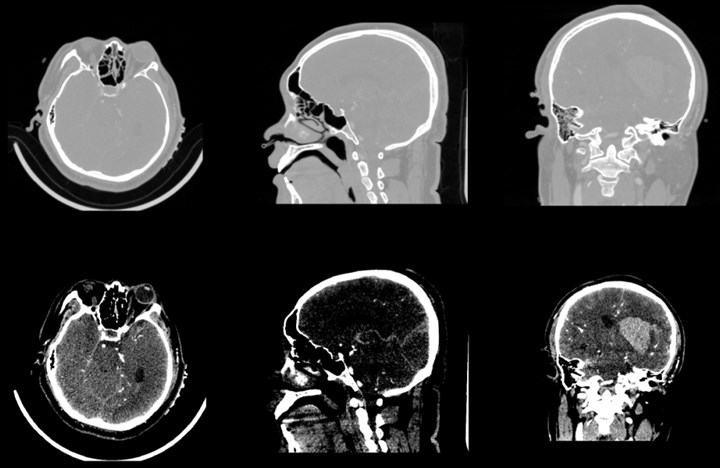
Fig. 4Commonly used grayscale preset
2.5. Volumes rendering
Volumes Rendering module provides interactive visualization of 3D image data. Only single-component scalar volumes can be used for volume rendering. Vector to scalar volume module can convert Vector volume to Scalar volume. Volume Rendering Module provides advanced tools for toggling interactive volume Rendering of datasets. If supported, Hardware accelerated volume rendering is available. The module permits selection of preset transfer functions to colorize and set opacity of data in a mission-appropriate way, and tools to customize the transfer functions that specify these parameters [4].
Open the eye button in front of the Volume and see that the 3D model of the brain has been reconstructed. The reconstruction process uses the GPU to achieve better image rendering. Preset: Apply a predefined set of functions to the opacity, color, and gradient transfer functions. Popularly speaking, the display methods for different tissues and organs are pre-set. For example, the head CTA has three presets: CT-Coronary-Arteries, CT-Coronary-Arteries-2, CT-Coronary- Arteries-3 is a preset scene dedicated to brain tissue or organs such as coronary arteries.
Fig. 5Select a preset window, after rendering selects VIK GPU ray casting
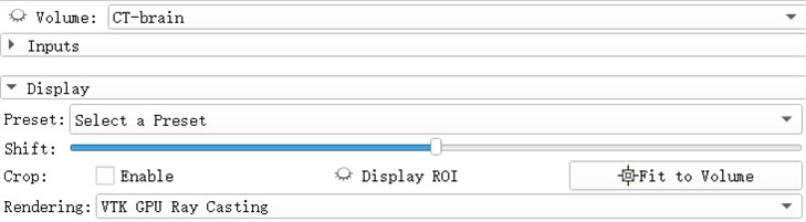
Fig. 6a) Default preset, b) CT coronary arteries – 3, capable of observing internal blood vessels and tissues, c) CT-Fat observes blood vessels like a perspective
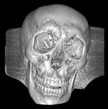
a)
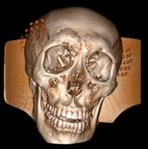
b)
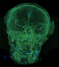
c)
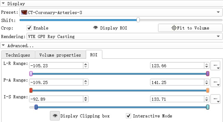
ROI (Region of Interest) can extract the regions of interest of the operator in the image. The region of interest of the 3d reconstruction model is composed of the ROI division regions in the direction of horizontal axis, sagittal axis and coronal axis. by adjusting the ROI range of a certain section, the change of the model can be observed. Light the eye before the Display ROI, so you can see the ROI check box in the model. Set the ROI precisely in the ROI TAB. Adjust the three slider positions to adjust ROI. When the Interactive Mode check box is checked, the adjustment of ROI will be reflected in the 3d view in real time.
3. Segments editor
Segments Editor Module can be selected in the process of hematoma modeling. This module allows editing segmentation objects by directly drawing and using segmentation tools on the contained segments. Representations other than the label map one (which is used for editing) are automatically updated real-time, so for example the closed surface can be visualized as edited in the 3D view. The module can adjust the display of the mask, opacity, outline display in the slice window, etc. The model can also be exported to Stl [5].
Open the Segments module, select the model to be modeled, add a mask, the color and name of the mask can be changed automatically. There is a variety of hematoma modeling methods, two of which are briefly introduced here. One is the threshold method, which is filled and segmented according to the model strength range, and the strength range can be adjusted by itself, and the hematoma can be independent with the choice of Islands. The other is the Fast Marching method, which can expand the selected part to the area with similar strength.
Fig. 7ROI parameter interface
3.1. Threshold
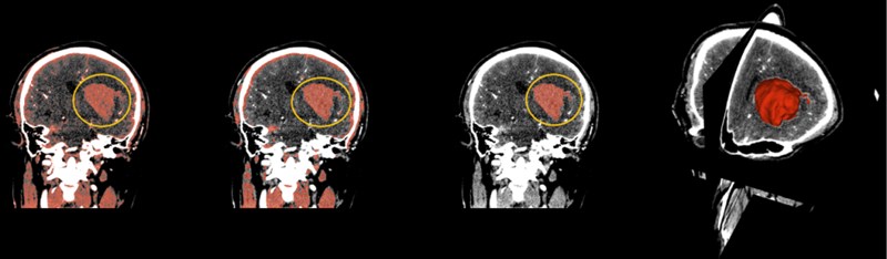
Select the Threshold function, which sets the selected intensity range to an editable intensity range for the mask, and then converts the masked area into a 3D model. For multiple small masks that appear in CT images, you can use the Smoothing feature to make the hematoma easier to separate by removing the stretched and filled holes to make the segmentation boundaries smoother. After smoothing, use the Islands function to separate the hematoma from the numerous masks. Select Keep selected island in the Islands function, click on the hematoma, and the hematoma is done independently.
Fig. 8(From left to right) The hematoma in the yellow circle is what we want to separate, using thresholding in the above order, then using smoothing to optimize staining, and finally using Islands to separate the hematoma. On the far right is the fusion of the hematoma and the three-dimensional map
3.2. Fast marching
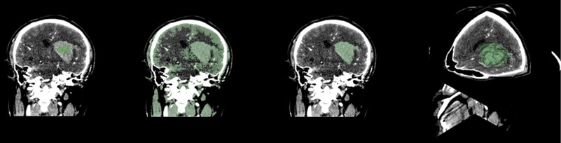
Select the Paint function to paint the hematoma area. Generally, the painting is painted in a plane. When using the rapid advance method, a spherical brush should be used. The brush is painted as a three-dimensional sphere, which is for subsequent Advancement is very helpful. After the painting is completed, open the Fast Marching function and select Initialize. After the initialization, the area around the hematoma is large. Adjust the segment of the Segment volume to reduce the mask and finally lock the position of the hematoma.
Fig. 9Fast marching renderings, faster than thresholding, but more computer-intensive
4. Skull stripper
Skull Stripper for MR/CT images of the brain. The algorithm registers a grayscale atlas image to the grayscale patient data. The associated atlas brain mask is propagated to the patient data using the registration transformation. This brain mask is eroded and serves as initialization for a refined brain extraction based on level-sets. The level-set towards the edge of the brain-skull border with dedicated expansion, curvature and advection terms [6].
Before selecting the module, it is necessary to import the CT or MR image data for skull exfoliation beforehand, and also import the Atlas and AtlasMask data for matching. After the import is complete, select the Swiss Skull Stripper module and select the corresponding data in the Altas column. After the basic operation is completed, click Apple to complete the skull stripping operation.
Fig. 10Corresponding to the writing of Altas data
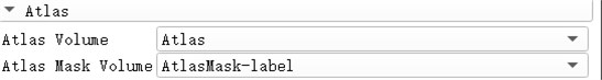
Fig. 11Above is the reference of the mask, below is the CT data we imported. It can be seen that the mask of the brain part of the CT data is very good, and the whole brain is isolated
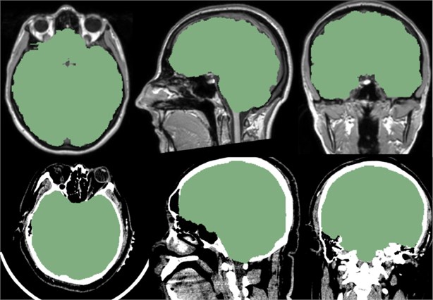
Fig. 12This is our independent brain mask in the Volumes Rendering module, CT-Fat preset. From these different perspectives, we can more clearly observe the blood vessels and tissues in the brain

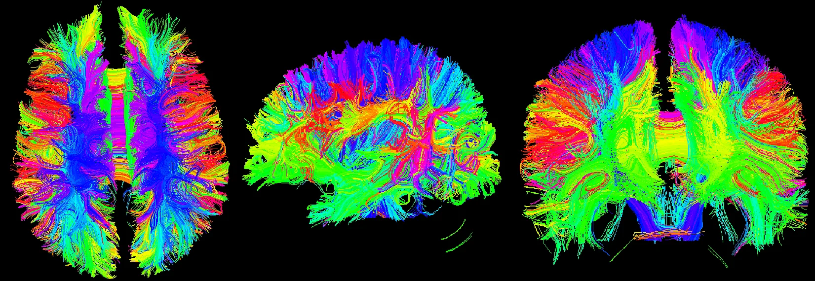
5. Neural fiber 3D modeling
5.1. Diffusion tensor image (DTI)
The physics of DTI is based on the dispersion of water molecules. Dispersion is a random and irregular free movement of water molecules – Brownian motion is one of the most basic physical phenomena. If the movement of water molecules is not restricted, then the movement of this three-dimensional motion in all directions is equal. This dispersion is called homomorphism. In human tissues, the movement of water molecules differs in all directions due to the influence of tissue cell structure. Therefore, it has the direction dependence, that is, it has the anisotropy. There are many parameters used to describe and analyze the degree of anisotropy, such as the Apparent Diffusion Coefficient (ADC), Mean Diffusivity (MD) and the Fractional Anisotropy (FA).
FA is the ratio of the anisotropy of water molecules to the total amount of diffusion. It is the most commonly used parameter. FA is sensitive to low anisotropy, and its size is closely related to the integrity of myelin sheath, fiber density and trend consistency, which can reflect the integrity of the white matter fiber bundle.
DTI belongs to brain function imaging which collects the motion information of water molecules in three-dimensional space. It can quantitatively analyze the dispersion characteristics of water molecules in tissues, measure the microstructure characteristics of white matter fibers, determine the spatial arrangement direction of white matter fiber bundles, and quantify to evaluate the heterogeneity of white matter, mainly used for the observation, tracking, brain development and brain cognitive function of white matter conduction bundles. Three-dimensional reconstruction using 3D Slicer shows the main white matter fiber bundles in the brain and identifies white matter fiber bundles in the brain. Anatomy, including contact fibers such as arcuate fibers, ligament bundles, superior longitudinal bundles, lower longitudinal bundles, upper frontal occipital bundles, lower frontal occipital bundles, anterior union, posterior combination, cerebellar midfoot, etc.; projection fibers such as corticospinal Bundles, lateral corpus callosum, cortical cerebellar tract, cortical pons, cortical nucleus, spinal thalamus bundle, spinal cord cerebellum bundle, etc. [7].
5.2. DWI converter
DWI belongs to the common diffusion-weighted imaging, only the diffusion coefficient is a scalar value used to describe the dispersion, but In DTI, the displacement of water molecules in a tissue is measured in at least six directions, and the tensor is essentially a vector diagram of the three-dimensional space. DTI is a more advanced form of diffusion-weighted imaging, new on the basis of DWI MR imaging technology, which uses a variety of parameters and data processing to reflect changes in the diffusion of imaging voxels in terms of quantity and direction, and can quantitatively and quantitatively evaluate the anisotropy of white matter.
However, the data required for DTI diffusion tensor fiber bundle imaging must be native DICOM data, rather than “semi-finished products” processed by the workstation. The processed data “Fa” can be directly applied, while the color DTI image cannot be applied. Of course, it is not ordinary diffusion-weighted scan data.
The correct file directory is selected for correct conversion, and we get a patient's data, often with many different kinds of scan sequences, all contained in a file directory, which can be independent using Mango software.
3D Slicer using DWI Converter module may be DTI DWI image conversion scan sequence is Nrrd format by parsing the header file to extract information on Measurement Frame, Diffusion Weighting Directions, sensitive to the diffusion coefficient value B-values and other necessary information to convert correctly. The converter currently supports data scanned by machines such as GE, Phillips, and Siemens [8].
5.3. Diffusion brain mask
Select the Diffusion Brain Masking module, which functions to create a brain mask in the DWI data obtained in the previous step, the diffusion weighted image. The mask can be used for diffusion tensor estimation or nerve beam imaging seeding. By averaging all baseline (non-diffusion weighted) images, the OTSU threshold algorithm was used to segment the tissue voxels, and then the small unconnected regions were removed to calculate the brain mask [9].
The main reason for generating the brain Mask is to narrow the scope of the FA map, which can remove the noise data outside the Mask, and thus can reduce the scope of the fiber bundle imaging, which not only reduces the workload but also makes the FA look more beautiful.
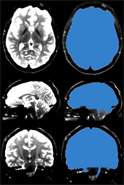
Fig. 13The brain mask, like the skull stripper, strips the brain from the skull, but the brain mask of the DWI data is prepared for the next step in generating DTI data
5.4. Diffusion tensor estimation
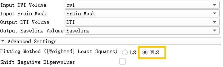
A diffusion tensor model is estimated from the diffusion-weighted image. There are two estimation methods available: least squares and weighted least squares. The least squares method is the traditional method of tensor estimation and the fastest method. The weighted least squares method takes into account the noise characteristics of the magnetic resonance image and weights the DWI samples according to their intensity [10].
Open the Diffusion Tensor Estimation module and insert DWI data and brain Mask to generate DTI data and reference volume data. Select WLS in the Fitting Method, which is Weighted Least Squares. The weighted least squares method is a mathematical optimization technique that weights the original model to make it a new model without heteroscedasticity and then estimates its parameters using ordinary least squares.
Fig. 14Generation of DTI data based on weighted least squares
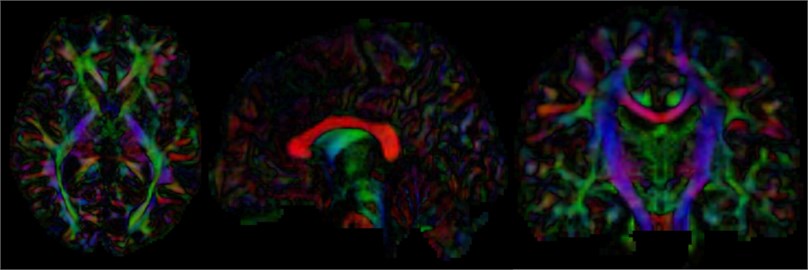
After calculating the diffusion tensor, the DTI data is obtained, and the three-dimensional map is browsed. It can be seen that the main dispersion direction red in the corresponding voxel indicates that the main feature vector of the voxel fiber bundle runs in the left and right direction. Green indicates that the main feature vector of the voxel fiber bundle travels in the front-rear direction. Blue indicates that the main feature vector of the voxel fiber bundle travels in the direction of the cephalopod.
Fig. 15Three-dimensional map of DTI data, the trend of the nerve bundle can be observed
5.5. Diffusion tensor soalar maps
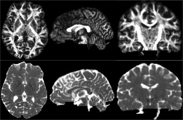
After the DTI image is obtained, the scalar measurement can be calculated therefrom. Available measurements include Fractional Anisotropy, Trace, and more. Open the Diffusion Tensor Soalar Maps module, enter the DTI data, export the scalar data from the tensor, enter “FA” if you select Fractional Anisotropy, or “Traces” if you select Traces. Select the Fractional Anisotropy and Traces parameters for the type of scalar measurement to be performed. Generate the corresponding parameters separately [11].
Fig. 16Three-dimensional map of fractional anisotropy and trace
5.6. Tracketography seeding
Tracketography Seeding module is used for interactive seeding of DTI fiber tracts starting from a list of fiducial points or vertices of a model or a label map volume. Select the existing DTI image data, and then select an existing benchmark. Point list, model or label mapping volume data as a seed, here select the Brain Mask volume data obtained by the brain virtual mask, and then obtain the nerve beam image of the whole brain [12].
Fig. 17Three-bit imaging of brain fiber bundles
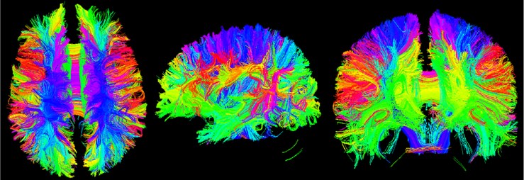
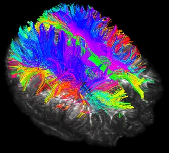
Fig. 18Fusion of brain fiber bundles and brain models of fractional anisotropy data in the volumes rendering module
Although the brain nerve bundle imaging is concrete and beautiful, it also has corresponding disadvantages. The rendering of the nerve bundle is too full, and we do not need all the nerve bundles in reality. Here we can selectively reconstruct by local seeding.
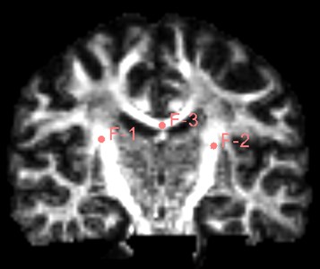
Find the Use mouse to Create-And-Place Fiducial icon in the toolbar and click to create a marker in the three-digit map. The maximum number of markers is 100, but generally not that much. Insert three markers here as an experiment.
Fig. 19Insert three marker points as shown
After inserting the marker point, open the Tracketography seeding module, the module will use the position of the marked point as the seed to grow the nerve bundle. After the Update option is allowed, when we freely move the marker point, the nerve bundle will grow in real time along with the marker point. The advantage of the seeding method is that we can adjust the position of the marker at any time, which is equivalent to the position, spacing and size of the nerve bundle growth at any time to meet the demand.
Fig. 20Tracketography seeding parameter interface, Fiducial Region Size controls the size of the fiber bundle, and the check mark before ‘Update’ allows the seed (marking point) to move freely as the seed (marking point) moves
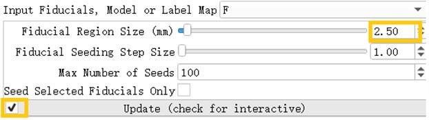
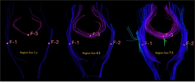
Fig. 21This is a bundle of different sizes, from left to right, 1.0 mm, 4.5 mm, 7.5 mm, you can see the importance of size for display
References
-
Yufu Cao Introduction of 3D Slicer. https://www.slicercn.com/?page_id=485, (in Chinese).
-
Mango Sofeware. Research Imaging Institute, UTHSCSA, http://rii.uthscsa.edu/mango/mango.html.
-
Pieper Steve, Finet Julien, Yarmarkovich Alex, Aucoin Nicole Volumes. https://www.slicer.org/wiki/Documentation/4.10/Modules/Volumes.
-
Finet Julien, Yarmarkovich Alex, Liu Yanling, Freudling Andreas, Kikinis Ron Volume Rendering. https://www.slicer.org/wiki/Documentation/4.10/Modules/VolumeRendering.
-
Csaba Pinter, Andras Lasso, Steve Pieper, Wendy Plesniak, Ron Kikinis, Jim Miller Segment Editor. https://slicer.readthedocs.io/en/latest/user_guide/module_segmenteditor.html.
-
Bauer S., Fejes T., Reyes M. A skull-stripping filter for ITK. Insight Journal, 2012, http://hdl.handle.net/10380/3353.
-
Cao Yufu DTI Tutorial 01-DTI Introduction and Software Installation. https://www.slicercn.com/?p=5318 (2018-07-28), (in Chinese).
-
Magnotta Vince DWI Converter. https://www.slicer.org/wiki/Documentation/4.10/Modules /DWIConverter.
-
Wassermann Demian, Norton Isaiah, O'donnell Lauren Diffusion Brain Masking. https://www.slicer.org/wiki/Documentation/4.10/Modules/DiffusionWeightedVolumeMasking#Information_for_Developers.
-
Jose Raul San, O'donnell Lauren, Wassermann Demian, Norton Isaiah, Yarmarkovich Alex Diffusion Tensor Estimation. https://www.slicer.org/wiki/Documentation/4.10/Modules /DWIToDTIEstimation.
-
Jose Raul San, O'donnell Lauren, Wassermann Demian, Norton Isaiah, Yarmarkovich Alex Diffusion Tensor Scalar Maps. https://www.slicer.org/wiki/Documentation/4.10/Modules /DiffusionTensorScalarMeasurements
-
Yarmarkovich Alex, Pieper Steve, Wassermann Demian, Norton Isaiah Tractography Interactive Seeding. https://www.slicer.org/wiki/Documentation/4.10/Modules/TractographyInteractiveSeeding.
Cited by
About this article

This work was supported by the National Science Foundation of China (51674121, 61702184), the Returned Overseas Scholar Funding of Hebei Province (C2015005014), the Hebei Key Laboratory of Science and Applications, and Tangshan Innovation Team Project (18130209B). Authors also thank Tangshan Gongren Hospital for their support of original data.
