Abstract
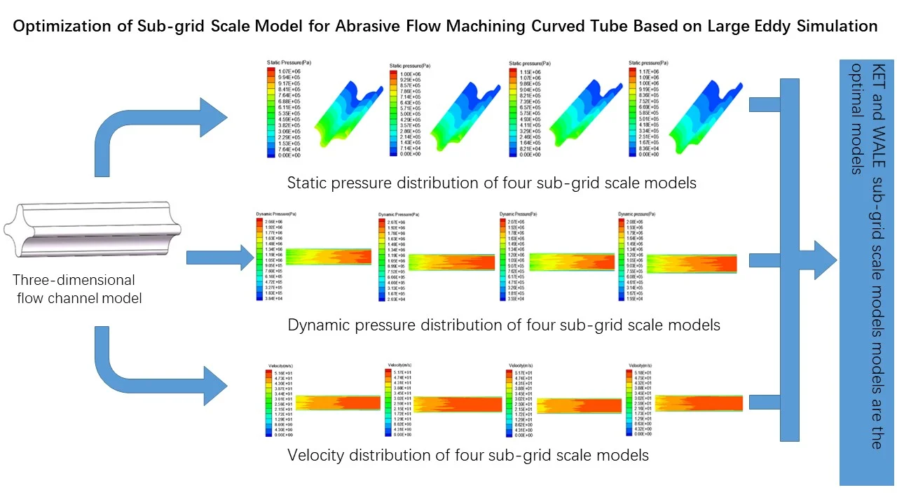
Abrasive flow machining technology is a new type of precision machining technology. Due to its unique rheological properties, it can process any complex structure and size parts to meet the requirements that conventional machining cannot meet. Combined with the turbulent flow characteristics of the abrasive flow, the large eddy simulation numerical method is used to simulate the machining process of the abrasive flow. The influence of different sub-grid scale models on the simulation results is discussed. Taking curved tube as the research object, the static pressure, dynamic pressure and velocity of different sub-grid models are analyzed to find the best sub-grid scale model. Large eddy simulation method is used to simulate the complex flow channel parts, and the best sub-grid scale model suitable for complex flow channels is determined, which reveals the grinding and polishing rule of abrasive flow and provides academic support for future research. Therefore, it has frontier and important research value.
Highlights
- For the complex flow channel, the curved tube is used to study the large eddy numerical simulation.
- The static pressure, dynamic pressure and speed of different sub-grid models are analyzed with curved tube as the research object.
- For the curved tube, the KET and WALE sub-grid scale models are more detailed for the faint flow of the fluid, and the large eddy simulation results are more accurate.
1. Introduction
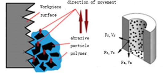
The core of the abrasive flow machining technology is the abrasive. The abrasive is mainly a solid-liquid two-phase flow composed of hard particles and liquid carriers. The processing of the abrasive flow is shown in Fig. 1. There are two forces in the force of the particles on the workpiece. Under the influence of external conditions, the particles follow the flow of the carrier to rub and shear the machined surface, thereby removing the burrs and obtaining a desired uniform surface.
The abrasive flow is a solid-liquid two-phase fluid. During the processing, its motion state is in the form of turbulent flow. By using the knowledge of fluid mechanics, an appropriate turbulence model is selected, and then the processing effect of abrasive particle flow is predicted by analyzing the flow field state and numerical value during the processing of abrasive particle flow.
Fig. 1Schematic diagram of abrasive flow polishing
2. Theoretical method of large eddy simulation
The large eddy simulation method was first proposed by meteorologist Smagorinsky [1] in 1963. The first use of this method was in 1970, Deardorff [2] in order to solve the engineering water flow problem. Later Ferziger introduced the turbulence kinetic energy and turbulence dissipation rate and took them into account the influence of vortex scale on vortex viscosity coefficient. Based on Smagorinsk formula, it was improved and corrected. Then Ghosal [3] discovered in 1995 that the model of Germano [4] had mathematical inconsistency in the application of heterogeneous isotropic, and then proposed a local dynamic model, and the eddy viscosity model was further developed.
The abrasive flow is in turbulent flow during motion. This is a three-dimensional unsteady irregular motion. The magnitude and direction of turbulent pulsation are random. Some parameters in the fluid, such as speed, temperature, concentration, and pressure, vary with time and space. Large-scale vortices slowly break down during the movement, gradually separating into small-scale vortices, and then separating them into smaller-scale vortices. The large-scale vortex carries the main energy, and the energy is transmitted to the small-scale vortex through the interaction between the vortices, and finally dissipated by the viscous fluid, and the small-scale vortex eventually disappears.
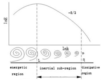
According to the energy transfer between the large-scale vortex and the small-scale vortex, the turbulent flow can be divided into two intervals: the energetic region and the dissipative region, and the corresponding feature scale is called the energetic scale L and the dissipative scale . In the high Reynolds number turbulence, the energetic zone and the dissipative zone are almost completely separated, so the interval between the energetic region and the dissipative region is called the inertial sub-region. The specific schematic diagram is shown in Fig. 2.
The basic idea of large eddy simulation is to solve the Navier-Stokes equation. Large eddy is directly solved, while small eddy needs to be modeled. In the large eddy simulation, the distinction between large-scale vortices and small-scale vortices is achieved by filtering. The small-scale vortex means that the feature scale is lower than the grid scale, and the model constructed in the solution process is also called the sub-grid scale (SGS) model.
The earliest sub-grid scale model Smagorinsky model was proposed in 1963 and was later developed by more researchers. The four common sub-grid models are Smagorinsky model, Wall-Adapting Local Eddy-viscosity (WALE) model, Algebraic Wall-Modeled LES (WMLES) model, and Dynamic kinetic Energy Sub-grid Scale (KET) model.
Fig. 2Schematic diagram of isotropic turbulent energy spectrum and feature scale
Among them are the Wall-Adapting Local Eddy-viscosity model and Algebraic Wall-Modeled LES [5]. The Smagorinsky model [1] is a pure dissipative model, and the Algebraic Wall-Modeled LES [6] uses Reynolds average method to simulate the flow field in the inner region of the boundary layer, while the large eddy simulation method is used outside the near wall region. Compared with the traditional algebraic model, the Dynamic kinetic Energy Sub-grid Scale model [7] increases the simulation of the turbulent kinetic energy transfer effect on the sub-grid scale.
3. Optimization of sub-grid scale model
In order to obtain high-precision simulation results of the abrasive flow machining curved tube, large eddy numerical analysis of the Smagorinsky model, the Wall-Adapting Local Eddy-viscosity (WALE) model, the Algebraic Wall-Modeled LES (WMLES) model, and the Dynamic Kinetic Energy Sub-grid Scale (KET) model are required respectively.
3.1. Establishment of three-dimensional model
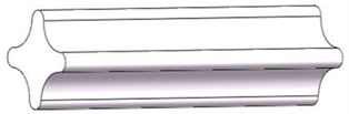
In the precise post-processing of internal curved surfaces in complex parts, the traditional machining method is difficult to perform precision machining. For such problems, the cycloidal parts are selected as the research object, and the parts are made of 304 stainless steel. In order to visually display the internal geometry of the flow channel of the simulation object, the flow channel is extracted in three dimensions, and the three structural parts have the same cross section dimension, and the flow channel geometry model and cross section specific dimensions are shown in Fig. 3 respectively.
Fig. 3Three-dimensional flow channel model
3.2. Static pressure distribution analysis of sub-grid scale model
The inlet is set as the pressure inlet of 2 MPa. The simulation results are studied and discussed to determine the appropriate sub-grid model and analyze the abrasive flow machining effect under different machining parameters. The straight flow channel is a symmetrical structure and the effect of the fluid on the wall surface is also symmetrical, so in order to facilitate the observation of the wall surface, half of the wall surface is selected for display. The static pressure distribution of the four sub-grid scale models is shown in Fig. 4.
Fig. 4Static pressure distribution of four sub-grid scale models
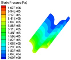
a) Smagorinsky model
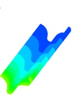
b) WALE model
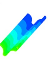
c) WMLES model
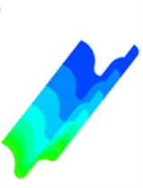
d) KET model
Fig. 4 is a static pressure distribution diagram of four sub-grid scale models using a large eddy simulation turbulence numerical method. The lower side of the figure is the inlet and the outer side is the outlet. The simulation results of the four sub-grid scale models show the same trend, and the pressure distribution presents a very obvious step shape, which indicates that the polishing effect of the abrasive flow is from strong to weak. The abrasive flow collides with the wall at the inlet, and most of the fluid flows away from the middle of the flow channel, which causes the contact force between the abrasive flow and the workpiece wall to slowly weaken and the pressure gradually decreases.
It can be seen from Fig. 4 that the simulation values of the four sub-grid scale models are different. The WALE sub-grid scale model has the smallest simulation value of 1 MPa and the KET sub-grid scale model has the largest simulation value of 1.17 MPa. It shows that the capture ability of the KET model is better than the other three sub-grid models, and combined with the polishing rule of the abrasive flow, within a certain range of pressure, the higher the polishing pressure is, the better the surface quality is obtained. Therefore, the KET model can be considered as a sub-grid scale model that meets our needs.
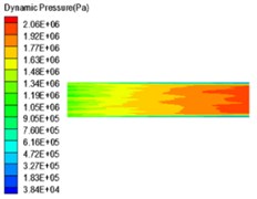
3.3. Dynamic pressure distribution analysis of sub-grid scale model
The abrasive flow is in a state of constant motion during the processing, so the dynamic pressure of the abrasive flow during the process is analyzed and discussed. In order to facilitate the observation of the change of the internal fluid, the cut surface is selected from the middle of the flow channel. In order to facilitate the description of the change of each position in the following, the cross section is described in position, and a specific schematic diagram is shown in Fig. 5. The position of the central section of the flow channel is 1-3, that is, the maximum width of the flow channel is 5mm, and the dynamic pressure under different sub-grid scale models is shown in Fig. 6.
Fig. 5Cross-sectional position division
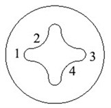
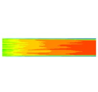
Fig. 6Dynamic pressure distribution of four sub-grid scale models
a) Smagorinsky model
b) WALE model
c) WMLES model
d) KET model
It can be seen from the dynamic pressure distribution of the four sub-grid scale models in Fig. 6 that the four dynamic pressure distributions have the same trend. It can be seen from Fig. 6 that it can be noticed at the wall that the dynamic pressure is a slowly decreasing process, indicating that the processing effect of the abrasive flow on the wall surface is gradually weakened. The abrasive flow rate between 2 and 4 in Fig. 5 is larger than the flow rate at the 1 position and the 3 position, the contact force between the abrasive flow and the wall surfaces 1 and 3 is weakened, and the dynamic pressure at the wall surface is reduced, indicating that the first half of the workpiece is better polished than the latter half, and further indicates that the polishing uniformity of the irregular inner curved surface by abrasive flow machining is slightly insufficient, and the polishing effect of positions 2 and 4 is better than that of positions 1 and 3.
3.4. Velocity distribution analysis of sub-grid scale model
The simulation results from Fig. 6 show that the simulation values of the four sub-grid scale models are basically the same, but there are still small deviations. According to the influence law of the polishing quality of the abrasive flow, the inlet pressure is proportional to the polishing quality within a certain range. The higher the pressure, the better the polishing quality of the abrasive flow. Therefore, KET sub-grid scale model is considered to be more suitable.
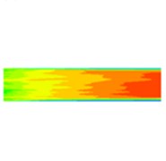
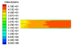
Fig. 7Velocity distribution of four sub-grid scale models
a) Smagorinsky model

b) WALE model
c) WMLES model

d) KET model
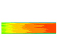
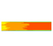
Fig. 7 shows the velocity distribution for the four sub-grid scale models. It can be seen from the figure that the simulation results of the four sub-grid scale models are also very similar. The higher the speed, the stronger the effect between the abrasive flow and the wall surface, and the greater the shear force of the abrasive flow to the wall surface, the better the polishing quality of the abrasive flow to the inner surface of the workpiece. At the outlet, the velocity in the middle of the flow channel is higher than near the wall surface, and green color exists on both sides of the red color, indicating that the flow velocity of the abrasive flow is on the same cross section, and the radial velocity is drastically reduced. This is mainly because the distance between the points on the special-shaped inner curved surface and the center of the flow channel is different in the axial section, and the abrasive flow rate at each position is different when the abrasive flow flows through the wall. The abrasive flow velocity is smaller at a wider position, and the abrasive flow velocity is larger at a narrower position, resulting in a reduction in wall shear force at positions 1 and 3, and a reduction in polishing quality and polishing uniformity.
4. Conclusions
Through the analysis of static pressure, dynamic pressure and speed parameters, it is found that the abrasive flow has better processing effect on the inlet and worse processing effect on the outlet, and the processing effects of positions 2 and 4 are better than positions 1 and 3. By analyzing the different sub-grid scale models, the numerical results of the KET sub- grid model are the largest, and the other three sub-grid scale models are relatively small, indicating that the KET sub-grid scale model can capture the maximum pulsation value of the flow field and has high simulation accuracy; The red positions of WALE and KET sub-grid scale models are found to be earlier than those of the other two sub-grid scale models through the velocity nephogram, indicating that the two sub-grid scale models can obtain small velocity transient changes in advance, and the capture capability is strong. Therefore, the KET and WALE sub-grid scale models can monitor the transient motion changes of the fluid in real time, capture the flow details of the flow field, and grasp the fluid flow's faint flow more carefully, and the large eddy simulation results are more accurate.
References
-
Smagorinsky J. General circulation experiments with the primitive equations I. The basic experiment. Monthly Weather Review, Vol. 91, Issue 3, 1963, p. 99-164.
-
Deardorff J. W. A numerical study of three-dimensional turbulent channel flow at large Reynolds numbers. Journal of Fluid Mechanics, Vol. 41, Issue 2, 1970, p. 453-480.
-
Ghosal S., Lund T. S., Moin P., et al. A dynamic localization model for large-eddy simulation of turbulent flows. Journal of Fluid Mechanics, Vol. 286, Issue 297, 1995, p. 229-255.
-
Germano M., Piomelli U., Cabot W. A dynamic subgrid-scale eddy viscosity model. Physics of Fluid, Vol. 3, Issue 3, 1991, p. 1760-1765.
-
Nicoud F., Ducros F. Subgrid-scale stress modelling based on the square of the velocity gradient tensor. Flow, turbulence and Combustion, Vol. 199, Issue 62, 3, p. 183-200.
-
Shur M. L., Spalart P. R., Strelets M. K., et al. A hybrid RANS-LES approach with delayed-DES and wall-modelled LES capabilities. International Journal of Heat and Fluid Flow, Vol. 29, Issue 6, 2008, p. 1638-1649.
-
Kim W. W., Menon S. Application of the localized dynamic subgrid-scale model to turbulent wall-bounded flows. AIAA Paper AIAA-97-0210, 1997.
About this article

The authors would like to thank the National Natural Science Foundation of China No. NSFC 51206011, Jilin Province Science and Technology Development Program of Jilin province No. 20170204064GX, Project of Education Department of Jilin province No. JJKH20190541KJ, Changchun Science and Technology Program of Changchun city No. 18DY017.
