Effect of public awareness, behaviours and treatment on infection-age-structured of mathematical model for HIV/AIDS dynamics

1. Introduction

Human Immunodeficiency Virus (HIV) Infection is a virus that destroys the immune system in an individual’s system which natural defence against illness. There are two types of HIV, which are HIV 1 and HIV 2, HIV 1 is the more fatal and deadly which is the cause of the Acquired Immunodeficiency Syndrome (AIDS) pandemic while, HIV 2 is also known to cause AIDS [1]. Symptoms of the virus are diarrheal, fever, constant cough, and skin problems usual infections, severe illnesses [2]. The virus infection spread from person to person including having unguarded sex with an infected person, sharing of the followings, needles, syringes as well as other items for injection drug use with an infected person. Blood transfusion or organ and tissue transplant can also transmit the virus [1]. The Virus does not spread through the following, skin to skin contact, shaking of hands, as well as kissing, through Air and water, drinking items, saliva, tears sharing of a toilet, towels and mosquitoes or insects biting [3].

There are stages of HIV infection which are Acute HIV infection is the first few weeks after infection. The second stage is called clinical latency is after the first month, HIV enters the clinical latency stage [3]. The third stage, AIDS which we called acquired immunodeficiency syndrome. Without treatment, HIV advance to AIDS, at this point, the immune system is too weak to fight off life-threatening disease and infection [1]. Whereas, untreated life expectancy with AIDS is about three years. HIV/AIDS destroys $T$ cells called CD4 cell, these cells help immune system fight infections of individuals. More so, healthy adults have a CD4 count of 800 to 1,000 per cubic millimetres. If CD4 count falls below 200 per cubic millimetres, then it is likely to have progressed to AIDS [3]. AIDS weakens the immune system to the point where it can no longer fight off most diseases and infections. This makes individuals more vulnerable to a wide range of illnesses [3].

Meanwhile, more than 70 million individuals have been infected with the HIV virus and about 35 million individuals have died of HIV [1]. Therefore, Sub-Saharan Africa remains most severely affected, with nearly 1 in every 25 adults (4.2 %) living with HIV. Mathematical models have been used frequently to study both transmission and infectious dynamics of virus [4]. Meanwhile, there are numerous works on Transmission of HIV/AIDS Infection. In this research work, we considered infection-age-structured of mathematical model of HIV/AIDS dynamics incorporating public awareness, behaviours and treatment.

2. Model formulation

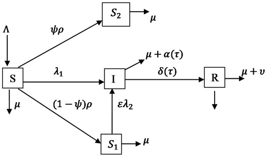
We considered an infection-age-structured mathematical model for transmission dynamic of HIV/AIDS infection incorporating HIV public awareness, sexual behaviours of some individuals and treatment. The transmission dynamics of HIV was developed using ordinary and partial differential equations and integro-differential equation. The total population ($N$) is partitioned into five (5) compartments, namely; unaware susceptible individuals ($S$), aware susceptible individuals whose modify their sex behaviours ($S_1$), aware susceptible individuals whose abstain and remain faithful to uninfected sex partners ($S_2$), infected individuals class ($I$) and removed individuals class ($R$).

$S\left(t\right)$ is generated by a recruitment rate of $\mathrm{\Lambda }$ and the natural death rate for all compartments is $\mu$. As a result of counselling and awareness, a proportion of the susceptible leave the $S$ class at the rate of $\psi$$(0<\psi <1)$which is the individuals abstained and remained faithful to uninfected sex partners and a fraction of $1-\psi$ is the rate at which individuals modify their sex behaviours. Also, $\rho$ is the rate $S$ of individuals knowing their HIV status. The expected reduction in unsafe sex behaviours by the $S_1$ class as a result of awareness is accounted for by $\epsilon$$(0<\epsilon <1)$. Thus, ${\lambda }_1$ is the force of infection from $S$ to $I$, where ${\lambda }_1={\beta }_{1}I\left(t\right)$ and ${\beta }_1$ is the incidence rate of unaware susceptible (effective infection contact rate). ${\lambda }_2$ is the force of infection from $S_1$ to $I$, where ${\lambda }_2={\beta }_{2}I\left(t\right)$ and ${\beta }_2$ is the incidence rate of aware susceptible. The infection spreads through direct contact between $S$ and $S_1$ with infected class ($I$). The disease induced death rate is $\alpha \left(\tau \right)$ and received treatment at the rate of $\delta \left(\tau \right)$, then moved to removed class ($R$), the $R$ class whose are assumed in this study not be involved in transmission as a result of efficacy of ART and has additional disease induced death rate of $\upsilon$, $I\left(t\right)$ is structured by the infection-age with the density function $i(t,\tau )$ following the idea of [3], where $t$ is the parameter and $\tau$ is the infection-age. There is a maximum infection age $T$ at which a number of the infected individuals form infected class leave the class via death, $0\le \tau \le T$. Meanwhile, since the infection period of HIV is long, then, the population is not constant, it is varying. A schematic diagram for the model is shown in Fig. 1.

Fig. 1Schematic diagram of HIV/AIDS infection

These assumptions lead to the following system of nonlinear integro-partial differential equations with non-local boundary conditions, which describes the dynamics of the transmission of the disease as:

where:

The total Population size $N$ is given by:

where:

Integration of Eq. (4) over $\tau$ is setting as:

Substituting Eqs. (8), (10) into Eq. (13) yields:

$T$ is the maximum infection age and if $\tau =T$ then the infected person die of the disease i.e.:

Implies:

3. Basic properties of the model

The addition of Eqs. (1), (2), (3), (5) and (16) is given by:

We apply theorem of differential inequality in [5] and separation of differential inequality of Eq. (18), we have:

Thus, as $t\to \infty$, we have:

Implies, as $\mathrm{l}\mathrm{i}\mathrm{m}t\to \infty$, $N\left(t\right)<\mathrm{\Lambda }/\mu$, where $N\left(0\right)<\mathrm{\Lambda }/\mu$.

However, if $N\left(0\right)\ge \mathrm{\Lambda }/\mu$, $N\left(t\right)$ will decrease to $\mathrm{\Lambda }/\mu$. So $N\left(t\right)$ is a bounded function of time. We can say that $\mathrm{\Omega }$ is bounded and at limiting equilibrium $t\to \infty$, $N\left(t\right)=\mathrm{\Lambda }/\mu$. Besides any sum or difference of variables in $\mathrm{\Omega }$ with positive initial values will remain in $\mathrm{\Omega }$ or in a neighbourhood of $\mathrm{\Omega }$. Thus $\mathrm{\Omega }$ is positively invariant and attracting with respect to the Eqs. (1)-(5) which are epidemiologically meaningful and mathematically well posed.

4. Existence and uniqueness of solution

We shall first and foremost establish the criteria for the existence and uniqueness of solution of the model Eqs. (4), (7) and (12). We define the derivative part of Eq. (4) as:

Let:

Then, the ordinary differential equation:

has the unique solution:

Using Eq. (23) in Eq. (25), we have:

which gives the value of $i$ at all point on the characteristics passing through the point $i(t_0,{\tau }_0)$, when $i(t_0,{\tau }_0)=(0,\tau -t)$; $h=t$, we have that:

Also, when $i(t_0,{\tau }_0)=(t-\tau ,0)$; $h=t$, we have:

The Eqs. (27) and (28) give the solution of $i(t,\tau )$ in the positive quadrant $t\ge 0$; $\tau \ge 0$.

Thus, problem Eqs. (4)-(12) has the following unique solution that exists for all time:

Eq. (29) is rewritten in the form:

where:

Eq. (31) denotes the survival probability, the probability for an individual to survive to age $\tau$; thus $\pi \left(\tau \right)=0$.

The expected life of an infected individual given by Eq. (26).

The function:

Let, $\varphi (•)$ is non-negative and belong to $L^T(0,\tau )$, $\alpha (•)$ is non-negative and belong to ${L^1}_{loc}\left(\right[0,\tau \left)\right)$, and

We rewrite Eq. (8) in the form:

where:

Eq. (35) are also non-negative and belongs to $L^T(0,\tau )$.

Substituting Eq. (30) into Eq. (34), we have for $t\le \tau$:

And for $t>\tau :$

Thus, $B\left(t\right)$ satisfies the following Volterra Integral equation of the second kind:

With:

where:

where $t\ge 0$ and the function $\phi ({\phi }_1,{\phi }_2)$, $\pi$ and $\varphi$ are extended by zero outside the interval [0, $T$]. Eq. (38) is known as the renewal equation and also as the Lotka equation, we observed that the kernel $K\left(t\right)$ is an infectious function of newly infected individuals defined in Eq. (32). Eq. (38) is equivalent to Eqs. (4), (8), and (12); actually Eq. (38) is the main tool to investigate the existence of Eqs. (4), (8) and (12), the connection being provided by Eqs. (30), (39) and (41) respectively. The following Lemma states some properties of Eq. (38) on the basis of the assumptions Eq. (33).

Lemma 1: Let Eq. (33) be satisfied, then:

If moreover, according to [6]:

Proof:

Eq. (42) and the first part Eq. (43) are obvious. To prove that $F\in \subset \left(R_{+}\right)$, we take $t_0\ge 0$ then we have:

where, $\varphi \in L^1\left(R\right)$:

As $t\to t_0$, so that:

Similarly, Eq. (44) implies $F\in W^{1,T}\left(R_{+}\right)$. Thus, completes the proof. In the next theorem, we establish the existence and uniqueness of Eqs. (4), (8) and (12) through Eq. (38). Now we study Eqs. (4), (8) and (12) by considering Eqs. (38)-(41). Since the function $F$ is continuous for the purpose of this section it is sufficient to study Eq. (38) in the class of continuous functions. Thus we introduce the following definition of a solution.

Definition 1. A Solution to Eq. (38) is a function $B\in \subset (R_{+},R)$ satisfying Eq. (38). First we have the following theorem, which is standard in the theory of Volterra equations. We provide a proof here for the sake of completeness.

Theorem 1. Let Eq. (33) be satisfied, then Eqs. (38)-(41) has a unique solution $B\in \subset (R_{+},R)$ such that $B\left(t\right)\ge 0$ for all $t$ in addition if $\varphi$ satisfied Eq. (44), then:

Proof: first we assume that:

The solution of Eq. (38) is obtained using the standard Picard iteration defined, for $t\ge 0$ by:

And initialized by $B^0\left(t\right)=0$ on IR⁺.

Therefore:

If we take any $T>0$, then by Eqs. (42)-(43) we obtained $B^k\in \left(\right[0,T\left]\right)$ and $B^k\left(T\right)\ge 0$, moreover:

Thus by Eq. (49) the sequence $B^k\left(t\right)$ converges uniformly on $[0,T]$ to a solution of Eq. (38) $∍B\in C\left(\right[0,T\left]\right)$ and $B\left(t\right)\ge 0$.

Concerning Uniqueness of this solution of the model, we set $B\left(t\right)$ and $\stackrel{-}{B}\left(t\right)$ to be the two solutions of Eq. (38), so that:

This implies that by Eq. (49), we have $B\left(t\right)=\overline{B}\left(t\right)$.

In addition, if $\varphi$ satisfied Eq. (44) then by Lemma 1 and Eq. (51), we have $B^k\in W^{1,T}\left(R_{+}\right)$ and setting $V^k\left(t\right)=\frac{d}{dt}{B}^k\left(t\right)$ a.e we have $V^k\in L^T\left(R_{+}\right)$ and

This yield:

Thus, again by Eq. (49) the sequence $V^k$ converges in $L^T\left(R_{+}\right)$ to $V\left(t\right)=\frac{d}{dt}B\left(t\right)$ are therefore Eq. (48) following from Eq. (55). In addition to Eq. (49), to make our argument valid we take $\alpha ∍$:

Setting $\overline{B}=e^{-\alpha t}B\left(t\right)$, $\overline{F}=e^{-\alpha t}F\left(t\right)$, $\overline{K}=e^{-\alpha t}K\left(t\right)$, Eq. (38) is transformed into an equation to the follows:

And since Eq. (58) satisfies Eq. (49), this is similar with Eq. (56). The next theorem allows us to state results for problem Eqs. (4), (8) and (12) through Eq. (30).

Theorem 2. Let Eq. (33) and Eq. (44) be satisfied, and we also assume that:

And let $i(t,\tau )$ defined by Eq. (30), where $B\left(t\right)$ is the solution of Eq. (38)-(40), then:

And problem Eqs. (4), (8) and (12) is satisfied. Moreover, according to [7], $i(t,\tau )$ is the only solution in the sense of Eqs. (60, 61).

Proof: the proof of Eqs. (60, 61) is quite straightforward and follows from the properties of $B\left(t\right)$ which is stated in Theorem 1. We only note the following inequality concerning the last part of Eq. (51):

Eq. (63) provides the fact that Eq. (59) is intended to guarantee the continuity of $i(t,\tau )$ through the line $\tau =t$; so that:

We note that the solution of problem Eqs. (4), (8) and (12) must be in the form of Eq. (30) with $B\left(t\right)$ satisfying Eqs. (38)-(40) such that Eqs. (30) and (44) are enough to provide a classical solution in the next following theorem.

Theorem 3. Let Eq. (33) be satisfied, then $i(t,\tau )$ defined by Eq. (30) has the following properties:

Proof: let us prove Eq. (66) first. From Eq. (39) we have:

Then, from Eq. (38):

Thus, by classical Gronwall’s inequality:

From this estimate, Eq. (30) yields:

Eq. (65) follows easily from Eq. (67). Now from a given $\varphi \in L^1(0,\tau )$, let ${\varphi }^n$ be a sequence such that ${\varphi }^n$ satisfy Eqs. (44) and (59):

And let $i^n$ be the solution of Eqs. (4), (8) and (12) corresponding to ${\varphi }^n$. Thus $i^n\in C\left(\right[0,T];L^1(0,\tau \left)\right)$ and by Eq. (66) and linearity, we have:

So that $i$ is the limit of the sequence $i^n$ in the Space $C\left(\right[0,T];L^1(0,\tau \left)\right)$ i.e Eq. (65) is true. Finally, Eqs. (67)-(68) are straightforward and that completes the proof.

This shows that even when the initial age of infection $\varphi$ is not regular the solution $i(t,\tau )$ still has some regularity. We also note that the estimate Eq. (66) provides continuity of the solution $i$with respect to initial age of infection $\varphi$. Hence, model Eqs. (4), (8) and (12) exist and are unique and well posed mathematically. In the norm of the space $L^1(0,\tau )$: this illustrates the existence and uniqueness of model Eqs. (4), (8) and (12) which is in agreement with the biological meaning of the age of infection $i(t,\tau )$ for the period of disease.

In the next theorem, we used a similar approach to the work of [2] to prove the existence and uniqueness of solution for the model Eqs. (1), (2), (3) and (5).

Theorem 4. The exists of a unique solution of Eqs. (1), (2), (3) and (5) for $\left|t-t_0\right|\le a$, $\left|S-S_0\right|\le b$, $\left|S_1-{S_1}_0\right|\le c,\left|S_2-{S_2}_0\right|\le d$, $\left|I-I_0\right|\le e$, $\left|R-R_0\right|\le f$.

Proof:

Then:

Taking the absolute (module) values of Eqs. (79-82) show that $\left|\frac{\partial f_i}{\partial x_j}\right|$, where $i=$ 1, 2, 3, 4 $\Rightarrow j=S,S_1,S_2,I,R$ are bounded. Hence, there is exists a unique solution of the model Eqs. (1-5).

5. Existence of equilibrium

Eqs. (1-5) are rewritten as follows:

At DFE, we let:

And set $\frac{dS}{dt}+\frac{d{S}_1}{dt}+\frac{d{S}_2}{dt}+\frac{dI}{dt}+\frac{dR}{dt}=0$, then we have the following results as the Disease Free Equilibrium (DFE):

6. Effective reproduction number

In an infection age and age-structured models, the basic or effective reproduction number are often expressed as the sum of the infectivity of each infected compartment, see for example in [8, 9]. For a single infected compartment, the basic reproduction number is simply the product of the infection rate and the mean duration of the infection, the effective reproduction number of the model becomes:

This is the number of secondary cases the number of generated by individuals in the actively infected class and $x^0=\left(\mathrm{\Lambda }/\mu +\rho \right)$ represents the number of susceptible individuals in the absence of HIV/AIDS. The term $\pi \left(\tau \right)=e^{-\underset{0}{\overset{\tau }{\int }}(\mu +\alpha (\tau )+\delta (\tau \left)\right)ds}$ is the survival probability as a function of infection age $\tau$ in the actively infected class. The effective reproduction number obtained in Eq. (92), using this to determine the Local Stability of the Disease Free Equilibrium State.

7. Local stability of the disease free equilibrium (DFE) state

Theorem 5. The DFE state $E^0$ is locally asymptotically stable if $R_E<\text{1}$ and unstable if $R_E>\text{1}$.

Proof: to show the local stability of DFE state given by Eq. (91), we have the following results:

Dividing both sides of Eq. (93) by $\overline{z}\left(0\right)$, we obtain:

where $x^0$ is defined as in Eq. (91).

Define a function $G\left(\lambda \right)$ to be right hand side in Eq. (94). $G\left(\lambda \right)$ is continuously differentiable function with $\mathrm{l}\mathrm{i}{\mathrm{m}}_{n\to \infty }G\left(\lambda \right)=0$ this shown that $G^1\left(\lambda \right)<0$ and therefore, $G\left(\lambda \right)$ is a decreasing function. Hence, any real solution of Eq. (94) is negative if $G\left(0\right)<\text{1}$ and positive if $G\left(0\right)>\text{1}$. Thus, if $G\left(0\right)>\text{1}$, then DFE state is unstable.

To show that Eq. (94) has no complex solution with non-negative real part if $G\left(0\right)<\text{1}$. In fact, we set:

Thus, we have:

Suppose $G\left(0\right)<0$. Assume that $\lambda =a_1+b_{1}i$ is a complex solution of Eq. (96) with $a_1\ge 0$ [7]:

It follows from Eq. (97) that Eq. (94) has solutions $\lambda =a_1+b_{1}i$ only if $a_1<0$. Thus, every solution of Eq. (94) must have a negative real part. We observed that $R_E=G\left(0\right)$. Therefore, the DFE state $E^0$ is locally asymptotically stable if $G\left(0\right)<\text{1}$.

8. Global stability of the disease free equilibrium (DFE) state

We construct a Lyapunov function as outline in the work of [10] to study the global stability of the DFE state in this study.

Theorem 6. The DFE state $E_0$ of the model Eqs. (1-5) is Globally Asymptotically Stable (GAS) in $\Omega$ if $R_E\le \text{1}$ while unstable if $R_E\ge \text{1}$.

Proof: Using the approach of [4], by constructing a suitable Lyapunov function as follows: