Modeling the effect of distancing and wearing of face masks on transmission of Covid-19 infection dynamics

Lasisi, Nurudeen O.; Adeyemo, Kolawole A.

doi:10.21595/chs.2021.21976

Journal of Complexity in Health Sciences

Browse Journal

Submit article

Published: 11 June 2021

Check for updates

Modeling the effect of distancing and wearing of face masks on transmission of Covid-19 infection dynamics

Nurudeen O. Lasisi¹

Kolawole A. Adeyemo²

¹Department of Statistics, Federal Polytechnic, Kaura Namoda, Nigeria

²Department of Computer Science and Mathematics, Nigeria Police Academy, Wudil, Nigeria

Corresponding Author:

Nurudeen O. Lasisi

Cite the article Download PDF

Downloads 851

CrossRef Citations 1

Abstract

The COVID-19 is an infection caused by corona virus which has been designated as pandemic in the word. In this paper, we proposed a model to study the effect of distancing and wearing of mask on transmission of Covid-19 infection dynamics. The invariant region of the model is established. The Covid-19 free equilibrium and the reproduction number of the model were obtained. The local and global stability of the model is determined using linearization technique method and Lyapunov method. It was found that, Covid-19 free equilibrium state is locally asymptotically stable in feasible region $Ω$ if $R_{0} < 1$ and globally asymptomatically stable if $R_{0} < 1$ , otherwise unstable if $R_{0} > 1$ . More so, numerical analysis and simulations of the dynamics of the Covid-19 infection are presented. It was found that as effectiveness of face mask usage increased it resulted in a decrease in secondary cases and as physical distancing is maintained shown reduction in reproduction number. It is also found that, as infection rate increases, it translated to increase in secondary cases and as number of isolation individual increases, it decreased the reproduction number. More so, varying the treatment rate, means as treatment rate increases, it shown that an individuals in the isolation decreases.

1. Introduction

The Covid-19 disease is an infectious disease caused by a newly revealed Corona virus [1]. Covid-19 characterised as asymptomatic or mild symptom to severe illness and mortality followed [2-5]. Corona viruses are large group of virus that cause mild to moderate high-respiratory tract illness, the main symptom are, fever, coughing, shortness of breath, trouble, breathing, fatigue, chills and shaking, body aches, headache, sore throat, loss of smell or taste, nausea, diarrhea [6]. The individuals infected with Covid-19 virus experienced mild to non-extreme respiratory illness and recover without requiring particular treatment [7-10]. People with ages and those with underlying health problems such as diabetes illness, cancer, and cardiovascular disease are more likely to develop serious illness [11, 12]. The most excellent way to prevent and slow down transmission is be well informed and educating about the Covid-19 virus, the disease it causes and how it spreads, it found that for people with mild disease, recover time is about two weeks, while people with severe or critical disease recover within three to six weeks [13-17]. As at now, there are no specific vaccinations or treatments for Covid-19. Meanwhile, there are numerous ongoing clinical trials evaluating potential treatments.

Mathematical models have played an indispensable role for understanding the dynamics of disease. Among the most popular are Ebola Virus [18] and The Human Immuno deficiency Virus (HIV) [19]. These models have been helpful to study the control and the transmission of the virus kinetics in order to provide a quantitative understanding and create public awareness of the virus, while [20] have designed mathematical models to explore the transmission dynamics and control of the Monkey-Pox infection. Hence, with the scarcity of data, the calculation, assumption and estimation of the values of the parameters of the model would be considered.

XGIJR model is an extension of standard SEIR model which we considered as more suitable for Covid-19 infection. In SEIR model, E is latent compartment denoted the individuals who are infected but not infectious. XGIJR model is the modification of SEIR model. In [21], the authors used SEIR model equations by incorporating time depend control and optimal control analysis. They used SEIR compartments to considered limited parameters, because they only focused at the trends, feeling, economic and political impacts caused by Covid-19 pandemic. The reality of Covid-19 was not considered as a compartment in SEIR model. In this case, our model considered the reality and mechanism of Covid-19 infection, which are Susceptible to the infection (S), Contact tracing (G) of individual, Infected individual (I), diagnosed and isolation of individual (J), and Recovered individual (R) and parameters such as, effectiveness of Mask usage and physical distancing. Even though there are still limitations on our work due to availability of data. Thus, give room for other to research and extend on.

2. Model formulation

A nonlinear mathematical model is proposed and analysed to study the effect of distancing and wearing of mask on transmission of Covid-19 infection dynamics. The proposed model subdivides the population of interest into five epidemiological compartments. In the modelling the Covid-19 dynamics, the population is divided into five subgroups: susceptible $X (t)$ , infective $I (t)$ , contact tracing $G (t)$ , isolation $J (t)$ , and recovery $R (t)$ . The susceptible are individuals that have not contracted the Covid-19 disease; Infective are individuals that have contracted the Covid-19 infection; Contact Tracing are individuals that have contact with infected person but have not being confirm of the infection; Isolation are individuals that have been confirmed of the infection and move to Isolation in order not to spread the disease, as shown in Fig. 1.

Fig. 1Schematic representation for the model equations

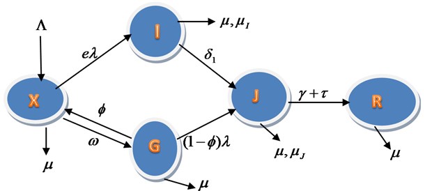
The transfer rates between the sub-groups indicating with tick arrows are collection of several epidemiological parameters. The susceptible population increase by recruitment rate $Λ$ and having the natural death rate $μ$ , Infection or Attack rate $α$ is the rate at which $X (t)$ is infected, $σ$ is the compliance of face mask usage and $ε$ is the practicing of the social and physical distancing, $ω$ is the unconfirmed contract tracing rate, $ϕ$ is the uninfected contact tracing return back to susceptible and ( $ϕ - 1$ ) is the proportion of contact tracing enter Isolation as a result of infection, $I (t)$ enter $J (t)$ with the rate of $δ$ and $J (t)$ enter $R (t)$ with the recovery parameters $γ$ and $τ$ . The rate of death due to Infection without isolation is $μ_{I}$ and Death rate due to Isolation is $μ_{J}$ .

Based on the above schematic representation and assumptions of the models, the equations governing the dynamics of the Covid-19 are given as:

1

\frac{d X}{d t} = Λ + ϕ G - \frac{e α I X}{N} - ω X - μ X,

2

\frac{d I}{d t} = \frac{e α I X}{N} - δ_{1} I - μ I - μ_{I} I,

3

\frac{d G}{d t} = ω X - ϕ G - (1 - ϕ) \frac{α I G}{N} - μ G,

4

\frac{d J}{d t} = δ_{1} I + (1 - ϕ) \frac{α I G}{N} - (γ + τ) J - (μ + μ_{J}) J,

5

\frac{d R}{d t} = γ J + τ J - μ R,

where, $e = (1 - ε) (1 - σ)$ .

3. Basic properties of the model

3.1. Invariant region

To obtain the invariant region, we considered the total human population ( $N$ ), where $N = X + I + G + Q + R$ . Then, the differentiation of N with respect to time leading to:

6

\frac{d N}{d t} = Λ + ϕ G - \frac{e α I X}{N} - ω X - μ X + \frac{e α I X}{N} - δ_{1} I - μ I - μ_{I} I + ω X - ϕ G

- (1 - ϕ) \frac{α I G}{N} - μ G + δ_{1} I + (1 - ϕ) \frac{α I G}{N} - (γ + τ) J - (μ + μ_{J}) J + γ J + τ J - μ R .

Eq. (6) gives as:

7

\frac{d N}{d t} = Λ - μ N - μ_{I} I - μ_{J} J .

In the absence of mortality due to Covid-19 infection ( $μ_{I} = μ_{J} = 0$ ), Eq. (7) yields:

8

\frac{d N}{d t} \leq Λ - μ N .

It follows from Eq. (8), the Gronwall inequality, that:

9

N (t) \leq N (0) e^{- μ (t)} + \frac{Λ}{μ} \{1 - e^{- μ (t)}\} .

$N (t) \leq Λ / μ$ if $N (0) \leq Λ / μ$ . Thus, $Ω$ is positively invariant. Hence, it is sufficient to consider the model dynamics Eqs. (1-5) in $Ω$ .

Theorem 1: (Invariant Region) the following biological feasible region of the model Eqs. (1-5), $Ω = \{(X, I, G, J, R) \in R^{5} : X (t) + I (t) + G (t) + J (t) + R (t) \leq \frac{Λ}{μ}\}$ is positive invariant and attracting.

3.2. Covid-19 free equilibrium (CFE)

The Covid-19 free equilibrium denoted by $E_{0}$ of the model system Eqs. (1-5) was obtained as:

10

(X^{0}, I^{0}, G^{0}, J^{0}, R^{0}) = (\frac{Λ (ϕ + μ)}{(ω + μ) (ϕ + μ) - ω ϕ}, 0,0, \frac{ω Λ}{(ϕ + μ) (ω + μ) - ω ϕ}, 0),

11

N^{0} = \frac{Λ (ϕ + μ) + ω Λ}{(ω + μ) (ϕ + μ) - ω ϕ} .

3.3. The basic reproduction number, $R_{0}$

Reproduction number $R_{0}$ is a process of measuring the transmission possible of disease. It is an average number of secondary infections produced by individual case of an infection in a population where everyone is susceptible. The basic reproduction number, $R_{0}$ of the model system Eqs. (1-5) is obtained by using the next generation operator method, approach of [21] and is given below:

12

R_{0} = \frac{(1 - ε) (1 - σ) α (ϕ + μ)}{(δ_{1} + μ + μ_{I}) [(ϕ + μ) + ω]} .

3.4. Local stability of Covid-19 free equilibrium

To determine the local stability of Covid-19 free equilibrium of the model system Eqs. (1-5) corresponding to Covid-19 free $E_{0}$ is obtained.

Theorem 2: If $R_{0} < 1$ , then the Covid-19 free equilibrium $E_{0}$ of the model system Eqs. (1-5) is locally asymptotically stable.

Proof: We used the linearization technique to determine the local stability of the Covid-19 free equilibrium $E_{0}$ , we have:

13

\begin{array}{l} H_{0} = J (X^{0}, I^{0}, G^{0}, J^{0}, R^{0}) \\ = (\begin{matrix} - \frac{e α I}{N} - ω - μ & - \frac{e α X}{N} & ϕ & 0 & 0 \\ \frac{e α I}{N} & \frac{e α X}{N} - δ_{1} - μ - μ_{I} & 0 & 0 & 0 \\ ω & - (1 - ϕ) \frac{α G}{N} & - ϕ - (1 - ϕ) \frac{α I}{N} - μ & 0 & 0 \\ 0 & δ_{1} + (1 - ϕ) \frac{α G}{N} & (1 - ϕ) \frac{α I}{N} & (- γ - τ - μ - μ_{J}) & 0 \\ 0 & 0 & 0 & γ + τ & - μ \end{matrix}) . \end{array}

At Covid-19 free equilibrium, we use Gaussian elimination row operation on Eq. (13) and the characteristic equation $|J (E_{0}) - λ I|$ is given as:

14

|J (E_{0}) - λ I| = (\begin{matrix} - P_{1} - λ & - \frac{e α X^{0}}{N^{0}} & ϕ & 0 & 0 \\ 0 & \frac{e α X^{0} - N^{0} P_{2}}{N^{0}} - λ & 0 & 0 & 0 \\ 0 & 0 & \frac{ϕ ω - P_{1} P_{3}}{P_{1}} - λ & 0 & 0 \\ 0 & 0 & 0 & - P_{4} - λ & 0 \\ 0 & 0 & 0 & 0 & - μ - λ \end{matrix}),

where, $P_{1} = ω + μ$ , $P_{2} = δ_{1} + μ + μ_{I}$ , $P_{3} = ϕ + μ$ , $P_{4} = γ + τ + μ + μ_{J}$ .

The characteristics equation corresponding to $H_{0}$ is:

15

|J (E_{0}) - λ I| = (- P_{1} - λ) (\frac{e α X^{0} - N^{0} P_{2}}{N^{0}} - λ) (\frac{ϕ ω - P_{1} P_{3}}{P_{1}} - λ) (- P_{4} - λ) (- μ - λ) = 0,

λ_{1} = - P_{1} = - (ω + μ) < 0,

λ_{2} = \frac{e α X^{0} - N^{0} P_{2}}{N^{0}} = \frac{e α X^{0} - N^{0} (δ_{1} + μ + μ_{I})}{N^{0}},

λ_{3} = \frac{ϕ ω - (ω + μ) (ϕ + μ)}{(ω + μ)} < 0, (ω + μ) (ϕ + μ) > ϕ ω,

λ_{4} = - P_{4} = - (γ + τ + μ + μ_{J}) < 0,

λ_{5} = - μ < 0 .

To confirm that $λ_{2} < 0$ , we have:

16

\begin{array}{l} λ_{2} = \frac{e α X^{0} - N^{0} (δ_{1} + μ + μ_{I})}{N^{0}} \\ = \frac{e α \frac{Λ (ϕ + μ)}{(ω + μ) (ϕ + μ) - ω ϕ} - \frac{Λ (ϕ + μ) + ω Λ}{(ω + μ) (ϕ + μ) - ω ϕ} (δ_{1} + μ + μ_{I})}{\frac{Λ (ϕ + μ) + ω Λ}{(ω + μ) (ϕ + μ) - ω ϕ}}, \end{array}

λ_{2} = \frac{[Λ (ϕ + μ) + ω Λ] (δ_{1} + μ + μ_{I}) [R_{0} - 1]}{Λ (ϕ + μ) + ω Λ},

λ_{2} = (δ_{1} + μ + μ_{I}) (R_{0} - 1) < 0, R_{0} < 1 .

Therefore, Covid-19 Free Equilibrium is locally asymptomatically stable if $R_{0} < 1$ and $(ω + μ) (ϕ + μ) > ϕ ω$ . So that infections do not persist in the population and under this condition the endemic equilibrium does not exist. It is unstable for $R_{0} > 1$ and endemic equilibrium exists and the Covid-19 infection is maintained in the population.

3.5. Global stability of Covid-19 free equilibrium

To prove global stability of the Covid-19 free equilibrium $E_{0}$ of the model Eqs. (1-5), we apply the approach by Castillo-Chavez (2002), by rewriting the model system Eqs. (1-5) as:

17

\frac{d K_{1}}{d t} = F (K_{1}, K_{2}),

\frac{d K_{2}}{d t} = H (K_{1}, K_{2}), H (K_{1}, 0) = 0,

where $K_{1} = (X^{0}, G^{0}, R^{0})$ and $K_{2} = (I^{0}, J^{0})$ , with the components of $K_{1} \in R^{3}$ denoting the uninfected groups and the components of $K_{2} \in R^{2}$ denoting the infected groups

The Covid-19 free equilibrium is now denoted as $E_{0} = (K_{1}^{*}, 0)$ , where $K_{1}^{*} = (N^{0}, 0)$ .

The two Conditions are:

– L1: $\frac{d K_{1}}{d t} = F (K_{1}, 0)$ .

– L2: $\hat{H} (K_{1}, K_{2}) = A K_{2} - H (K_{1}, K_{2})$ .

Theorem 3: If $R_{0} < 1$ , the Covid-19 free equilibrium $E_{0}$ of the model system Eqs. (1-5) is globally asymptotically stable (GAS) in $Ω$ .

Proof: To establish the global stability of Covid-19 free equilibrium $E_{0}$ , the two conditions (L1) and (L2) as in Castillo-Chavez (2002) must hold for $R_{0} < 1$ .

Now, for the first condition, that is global asymptotic stability of $K_{1}^{0}$ , gives:

18

\frac{d K_{1}}{d t} = F (K_{1}, 0) = [\begin{matrix} Λ + ϕ G^{0} - ω X^{0} - μ X^{0} \\ ω X^{0} - ϕ G^{0} - μ G^{0} \\ - μ R^{0} \end{matrix}] .

Solving linear differential equations of Eq. (18), we have:

19

X^{0} (t) = \frac{Λ + ϕ G^{0}}{(ω + μ)} - \frac{Λ + ϕ G^{0}}{(ω + μ)} e^{- (ω + μ) t} + X^{0} (0) e^{- (ω + μ) t},

G^{0} (t) = \frac{ω X^{0}}{(ϕ + μ)} - \frac{ω X^{0}}{(ϕ + μ)} e^{- (ϕ + μ) t} + G^{0} (0) e^{- (ϕ + μ) t},

R^{0} (t) = R^{0} (0) e^{- μ t} .

Now, clearly Eq. (10) gives $[X^{0} (t) +, G^{0} (t) +, R^{0} (t)] \to N^{0} (t)$ as $t \to \infty$ regardless of the value of $X^{0} (t)$ , $G^{0} (t)$ and $R^{0} (t)$ . Thus, $K_{1}^{*} = (N^{0}, 0)$ is globally asymptotically stable.

Next, for the second condition, that is $\hat{H} (K_{1}, K_{2}) = A K_{2} - H (K_{1}, K_{2})$ , gives:

20

A = (\begin{matrix} \frac{e α X^{0}}{N^{0}} - (δ_{1} + μ + μ_{I}) & 0 \\ δ_{1} + (1 - ϕ) \frac{α G^{0}}{N^{0}} & - (γ + τ + μ + μ_{J}) \end{matrix}),

H (K_{1}, K_{2}) = (\begin{matrix} \frac{e α I^{0} X^{0}}{N^{0}} - (δ_{1} + μ + μ_{I}) I^{0} \\ δ_{1} I^{0} + (1 - ϕ) \frac{α I^{0} G^{0}}{N^{0}} - (γ + τ + μ + μ_{J}) J^{0} \end{matrix}) .

Therefore:

21

\hat{H} (K_{1}, K_{2}) = A K_{2} - H (K_{1}, K_{2})

= (\begin{array}{l} \frac{e α X^{0}}{N^{0}} - (δ_{1} + μ + μ_{I}) & 0 \\ δ_{1} + (1 - ϕ) \frac{α G^{0}}{N^{0}} & - (γ + τ + μ + μ_{J}) \end{array}) (\begin{array}{l} I^{0} \\ J^{0} \end{array})

- (\begin{matrix} \frac{e α I^{0} X^{0}}{N^{0}} - (δ_{1} + μ + μ_{I}) I^{0} \\ δ_{1} I^{0} + (1 - ϕ) \frac{α I^{0} G^{0}}{N^{0}} - (γ + τ + μ + μ_{J}) J^{0} \end{matrix})

= (\begin{matrix} \frac{e α X^{0} I^{0}}{N^{0}} - (δ_{1} + μ + μ_{I}) I^{0} & 0 \\ δ_{1} + (1 - ϕ) \frac{α I^{0} G^{0}}{N^{0}} & - (γ + τ + μ + μ_{J}) J^{0} \end{matrix})

- (\begin{matrix} \frac{e α I^{0} X^{0}}{N^{0}} - (δ_{1} + μ + μ_{I}) I^{0} \\ δ_{1} I^{0} + (1 - ϕ) \frac{α I^{0} G^{0}}{N^{0}} - (γ + τ + μ + μ_{J}) J^{0} \end{matrix})

= (\begin{array}{l} 0 \\ 0 \end{array}) \hat{H} (K_{1}, K_{2}) = A K_{2} - H (K_{1}, K_{2}) = (\begin{array}{l} 0 \\ 0 \end{array}),

i.e $\hat{H} (K_{1}, K_{2}) = {(0,0)}^{T}$ .

It is thus obvious that $\hat{H} (K_{1}, K_{2}) = 0$ . Hence, the proof is complete. Therefore, Covid-19 free equilibrium is globally asymptomatically Stable in the feasible region $Ω$ if $R_{0} < 1$ .

4. Numerical simulations

According to Nigeria Centre for Disease Control (NCDC) reported on 17th June, 2020 on Covid-19 updated, total cumulative tested person is 103,799; total cumulative infected cases is 17,735; total cumulative recovered cases is 5,967; total cumulative death is 469 and we assumed the number of the contact tracing is 200,000. We calculate and estimate the parameters values based on the availability of information from the aforementioned organization. The reasons for the values are obviously explained in details in the following statements. According to the available data, 80 % of total death resulted to death due to Disease without quarantine in Nigeria, however, due to the overwhelmed and poor medical infrastructure and 20 % of total death resulted to death due to quarantine.

Total population = $X (t) + [I (t) + J (t)] + G (t) + R (t)$ , where, $X (t) =$ 200,000,000 – [7,735 + 10,000] – 200,000 – (5,967 + 469) = 199,775,829.

Recovery rate ( $γ$ ) = number of recovery / number of cases.

Infection or attack rate ( $α$ ) = number of new cases in population at risk / number of persons at risk in the population.

Disease death rate = number of death from Covid-19 infection/ total number of cases death rate due to infection ( $μ_{I}$ ).

Contact tracing rate ( $ω$ ) = number of tracing or sample tested / total population of the area.

Uninfected contact tracing rate ( $ϕ ω$ ) = number of contact tracing tested but uninfected / total number tested for Covid-19.

Table 1Values for variables and parameters of the model

Parameters	Definitions	Values
$Λ$	Recruitment rate	271.23/day
$σ$	Usage of face mask	{0, 1}
$ε$	Practicing social and physical distancing	{0, 1}
$ϕ$	Uninfected contact tracing rate	0.83/day
$ω$	Contact tracing rate	0.00052/day
$α$	Infection or attack rate	0.001/day
$γ$	Recovery rate	0.336/day
$τ$	Booster	{0,0.5}
$δ$	Movement rate from $I$ to $J$	Assumed (0.6)
$μ$	Natural death rate	0.0017/day
$μ_{I}$	Death rate due to infection	0.0212/day
$μ_{J}$	Death rate at isolation centre	0.0053/day
$N$	Total population number	200,000,000

The data for numerical simulations of $R_{0}$ with respect to each of the epidemic parameters are given in Table 1 and Using Maple 17 Software for the graphical representation of reproduction numbers and model simulations with parameter values of the model equations are sin Figs. 2-3.

Fig. 2 shows the effect of face masks usage in reducing the spread of Covid-19 infection. It is shown that as the use of face mask increases it is resulted to decrease in reproduction number (secondary cases). Thus, varying the social and physical distancing, we observed that reproduction number reduced significantly.

Fig. 3 showed that as uninfected contract tracing increases, it is also increased the reproduction number, this is because, as the uninfected contact tracing reappear into population, it increased the secondary cases and make individual more susceptible to the infection. Meanwhile, varying the contact rate we found that as contact rate increases, it increased the secondary cases.

It is observed from Fig. 4 that as the infection rate (attack rate) increases, it is translated to increase on reproduction number (secondary cases), also as contact tracing rate increase, the reproduction number decreased.

Fig. 5 shows that as rate of isolation increases, it decreased the reproduction number, varying the death rate due to Covid-19 infection without isolation, we found that as death rate due to Covid-19 infection without isolation increases, it decreased the reproduction number.

Fig. 2Effect of face masks usage on reproduction number on reproduction number (R0)

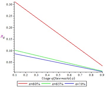
Fig. 3Effect of uninfected contact tracing on reproduction number (R0)

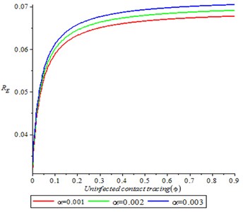
Fig. 4Effect of infection rate on reproduction number (R0)

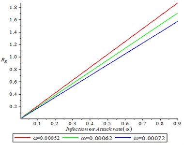
Fig. 5Effect of rate of I to J on reproduction number (R0)

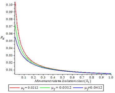
Fig. 6Variation of proportion of contact tracing for different values of ω, ε

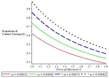
a)

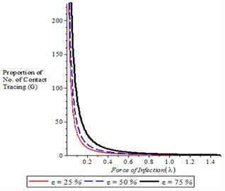
b)

Fig. 6(a) shows that as the proportion of contract tracing increases, it is translated to decrease in force of infection. It is also observed from Fig. 6(b) that as number of complier in physical distancing increases, it is resulted in decrease in force of infection.

Fig. 7, shown the dynamics of population of isolation, it is observed that the number of isolation individuals increases with time, varying treatment rate. It means as treatment rate increased, it is seen the individuals in the isolation decreases.

Fig. 8 shown the dynamics of Recovered person with time, with different rate, it is observed from the simulation, that as recovery rate increases, it is translate to increase in recovery individual.

Fig. 9 shows the proportion of three populations, it is observed that the proportion of infective population increase to a pick before started decreasing as a result of isolation of infected person. The process of contact tracing is not encouraging as it shown in simulation.

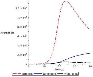
It is observed from Fig. 10, that as infected person reached it pick, the isolation and recovery individual started increasing which resulted to decreased in infected person.

Fig. 7Population of isolation for different values of treatment,τ

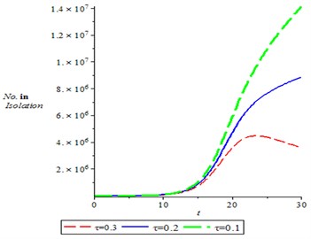
Fig. 8Recovery individual population for different values of γ

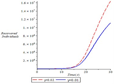
Fig. 9Variation of proportion of total population in different classes (infected, contact tracing and isolation)

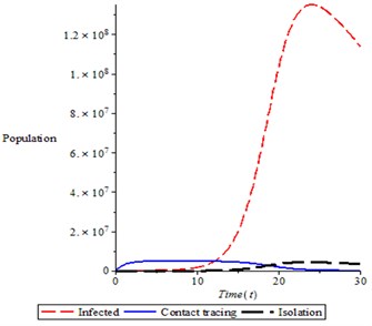
Fig. 10Variation of total population in different classes (infected, recovered and isolation)

5. Conclusions

A nonlinear mathematical model has been proposed and analysed to study the effect of distancing and wearing of masks on transmission of Covid-19 infection dynamics in a population. The invariant region of the model was established. The Covid-19 free equilibrium state was obtained and the stability of Covid-19 free equilibrium was investigated. The model showed that the Covid-19 free equilibrium is locally stable using linearization technique method at threshold parameter less than unity and unstable at threshold parameter greater than unity. The global stability of Covid-19 free equilibrium state was established, by the construction of Lyapunov method, it was showed that Covid-19 free equilibrium is globally asymptomatically stable in the feasible region $Ω$ if $R_{0} < 1$ . Based on the results of the study and simulations, we conclude that the most effective way to reduce the transmission of Covid-19 Infection is to educate individuals on the use of face masks and sustain physical distancing, because use of face mask reduced the spread of Covid-19 infection and physical distancing also reduced the number of secondary cases. More so, as isolation rate increased, it depleted the reproduction number and as treatment rate increased, it is seen that the individuals in the isolation decreased. Finally, there is need for further research work on the effect of asymptomatic and symptomatic on the spread of the disease, vaccination and other control strategies should be consider in controlling the spread of Covid-19 infection.

References

Y. Li, et al., “Mathematical modeling and epidemic prediction of COVID-19 and its significance to epidemic prevention and control measures,” Annals of Infectious Disease and Epidemiology, Vol. 5, No. 1, 2020, p. 1052.

Search CrossRef
Z. J. Cheng and J. Shan, “2019 Novel coronavirus: where we are and what we know”, Infection Journal, Vol. 48, No. 2, pp. 155–163, 2020, https://doi.org/10.1007/s15010-020-01401-y

Publisher
Q. Li, et al., “Early transmission dynamics in Wuhan, China, of novel coronavirus-infected pneumonia,” New England Journal of Medicine, Vol. 382, No. 13, pp. 1199-1207, 2020, https://doi.org/10.1056/NEJMoa2001316

Publisher
C. Rothe, et al. “Transmission of 2019-nCoV Infection from an asymptomatic contact in Germany”, New England Journal of Medicine, Vol. 382, No. 10, pp. 970–971, 2020, https://doi.org/10.1056/NEJMc2001468

Publisher
A. Sahin, et al. “2019 novel coronavirus (COVID-19) outbreak: A review of the current literature”, Eurasian Journal of Medicine and Oncology, Vol. 4, No. 1, pp. 1–7, 2020, https://doi.org/10.14744/ejmo.2020.12220

Publisher
“WHO statement regarding cluster of pneumonia cases in Wuhan, China,” 2020, https://www.who.int/china/news/detail/09-01-2020-\who-statement-regarding-cluster-of-pneumonia-cases-in-wuhan-china

Search CrossRef
J. M. Read, J. R. E. Bridgen, D. A. T. Cummings, A. Ho, and C. P. Jewell, “Novel coronavirus 2019-nCoV: early estimation of epidemiological parameters and epidemic predictions”, medRxiv, Vol. 1, No. 1, 2020, p. 234, https://doi.org/10.1101/2020.01.23.20018549

Publisher
B. Tang, et al., “Estimation of the transmission risk of 2019-nCoV and its implication for public health interventions”, Journal of Clinical Medicine, Vol. 9, No. 2, 2020, p. 462, https://doi.org/10.3390/jcm9020462

Publisher
N. Imai, et al., “Report 3: Transmissibility of 2019-nCoV”, Reference Source, 2020, https://www.imperial.ac.uk/mrc-global-infectious-disease-analysis/news--wuhan-coronavirus

Search CrossRef
H. Zhu, et al., “Host and infectivity prediction of Wuhan 2019 novel coronavirus using deep learning algorithm”, Mathematical Biosciences and Engineering Vol. 17, No. 3, pp. 2708–2724, 2020.

Search CrossRef
“WHO novel coronavirus (2019-nCoV) situation reports”, https://www.who.int/emergencies/diseases/novel-coronavirus-2019/situation-reports

Search CrossRef
“Centers for Disease Control and Prevention: 2019 novel coronavirus”, https://www.cdc.gov/coronavirus/2019-ncov

Search CrossRef
P. Zhou, et al., “Discovery of a novel coronavirus associated with the recent pneumonia outbreak in humans and its potential bat origin”, bioRxiv, 2020, https://doi.org/10.1101/2020.01.22.914952

Publisher
L. E. Gralinski, and V. D. Menachery, “Return of the coronavirus: 2019-nCoV,” Viruses, Vol. 12, No. 12, 2020, p. 135, https://doi.org/10.3390/v12020135

Publisher
V. J. Munster, M. Koopmans, N. V. Doremalen, D. V. Riel, and E. D. Wit, “A novel coronavirus emerging in China – key questions for impact assessment”, New England Journal of Medicine, Vol. 382, pp. 692–694, 2020, https://doi.org/10.1056/NEJMp2000929

Publisher
C. Geller, M. Varbanov, and R. E. Duval, “Human coronaviruses: Insights into environmental resistance and its influence on the development of new antiseptic strategies”, Viruses, Vol. 4, pp. 3044–3068, 2012, https://doi.org/10.3390/v4113044

Publisher
J.-T. Wu, K. Leung, and G. M Leung, “Nowcasting and forecasting the potential domestic and international spread of the 2019-nCoV outbreak originating in Wuhan, China: a modelling study”, Lancet, Vol. 395, pp. 689–697, 2020, https://doi.org/10.1016/S0140-6736(20)30260-9

Publisher
N. O. Lasisi et. al., “Mathematical model for Ebola virus infection in Human with effectiveness of drug usage”, Journal of Applied Science Environmental Management, Vol. 22, No. 7, pp. 1089–1095, 2018, https://dx.doi.org/10.4314/jasem.v22i7.16

Publisher
N. O. Lasisi, “Effect of public awareness, behaviours and treatment on infection-age-structured of mathematical model for HIV/AIDS dynamics”, Journal of Mathematical Models in Engineering, Vol. 6, No. 2, p. 103–121, 2020, https://doi.org/10.21595/mme.2020.21249

Publisher
N. O. Lasisi, N. I. Akinwande, and F. A. Oguntolu, “Development and exploration of a Mathematical Model for Transmission of Monkey-Pox in Humans”, Journal of Mathematical Models in Engineering, Vol. 6, No. 1, pp. 23–33, 2020, https://doi.org/10.21595/mme.2019.21234

Publisher
N. O. Lasisi, N. I. Akinwande, and S. Abdulrahaman, “Optimal Control and Effect of Poor Sanitation on Modeling the Acute Diarrhea Infection”, Journal of Complexity in Health Sciences, Vol. 3, No. 1, pp. 91–103, 2020, https://doi.org/10.21595/chs.2020.21409

Publisher
H. T. Alemneh and G. T. Tilahun, “Mathematical modeling and optimal control analysis of COVID-19 in Ethiopia,” medRxiv, July 24, 2020, https://doi.org/10.1101/2020.07.23.20160473

Publisher

Cited by

A General Epidemic Model and Its Application to Mask Design Considering Different Preferences towards Masks

Chaoqian Wang | Hamdi Kavak | Roberto Natella

(2022)

About this article

Received

04 April 2021

Accepted

04 May 2021

Published

11 June 2021

DOI

https://doi.org/10.21595/chs.2021.21976

Keywords

distancing

reproduction number

wearing of mask

local and global stability

modelling

transmission

This is an open access article distributed under the Creative Commons Attribution License, which permits unrestricted use, distribution, and reproduction in any medium, provided the original work is properly cited.

Previous article in issue Previous Next article in issue Next

Research article

2023 10 31

Dynamic characteristics analysis for gear transmission system in shearer cutting section under different loads

Guo Ye, Xing Deng, Jinyong Ju, Lianchao Sheng

Research article

2023 05 18

Enhancing model estimation accuracy and convergence rate in hysteresis modeling of MFC actuators using modified differential evolution algorithm

Hafiz Muhammad Umar, Ruichen Yu, Zhiyuan Gao, Hesheng Zhang

Research article

2021 09 13

Convolutional mask-wearing recognition algorithm for an interactive smart biometric platform

Patryk Bałazy, Paweł Gut, Paweł Knap

Research article

2021 06 21

Lyapunov approach and global stability of Ebola virus infection model of an individual cells population

Nurudeen Oluwasola Lasisi

N. O. Lasisi and K. A. Adeyemo, “Modeling the effect of distancing and wearing of face masks on transmission of Covid-19 infection dynamics,” Journal of Complexity in Health Sciences, Vol. 4, No. 1, pp. 10–20, Jun. 2021, https://doi.org/10.21595/chs.2021.21976

Copy Extrica

Copied to clipboard!

TY  - JOUR
DO  - 10.21595/chs.2021.21976
UR  - https://doi.org/10.21595/chs.2021.21976
TI  - Modeling the effect of distancing and wearing of face masks on transmission of Covid-19 infection dynamics
T2  - Journal of Complexity in Health Sciences
AU  - Lasisi, Nurudeen O.
AU  - Adeyemo, Kolawole A.
PY  - 2021
DA  - 2021/06/11
PB  - JVE International Ltd.
SN  - 2538-7995
SN  - 2538-8002
ER  - 

Copy Ris

Copied to clipboard!

@article{Lasisi_2021,
	doi = {10.21595/chs.2021.21976},
	url = {https://doi.org/10.21595/chs.2021.21976},
	year = 2021,
	month = {jun},
	publisher = {{JVE} International Ltd.},
	author = {Nurudeen O. Lasisi and Kolawole A. Adeyemo},
	title = {Modeling the effect of distancing and wearing of face masks on transmission of Covid-19 infection dynamics},
	journal = {Journal of Complexity in Health Sciences}
}

Copy Bibtex

Copied to clipboard!

[1]N. O. Lasisi and K. A. Adeyemo, “Modeling the effect of distancing and wearing of face masks on transmission of Covid-19 infection dynamics,” Journal of Complexity in Health Sciences, Jun. 2021, doi: 10.21595/chs.2021.21976.

Copy IEEE

Copied to clipboard!

Lasisi, Nurudeen O., and Kolawole A. Adeyemo. “Modeling the Effect of Distancing and Wearing of Face Masks on Transmission of Covid-19 Infection Dynamics.” Journal of Complexity in Health Sciences, June 11, 2021. https://doi.org/10.21595/chs.2021.21976.

Copy Chicago

Copied to clipboard!

Modeling the effect of distancing and wearing of face masks on transmission of Covid-19 infection dynamics

Abstract

1. Introduction

2. Model formulation

3. Basic properties of the model

3.1. Invariant region

3.2. Covid-19 free equilibrium (CFE)

3.3. The basic reproduction number, R0

3.4. Local stability of Covid-19 free equilibrium

3.5. Global stability of Covid-19 free equilibrium

4. Numerical simulations

5. Conclusions

References

Cited by

About this article

Related Articles

3.3. The basic reproduction number, $R_{0}$