Abstract
In this paper, an analytical method is developed for the calculation of control forces to create stationary points, called nodes, at desired locations in a vibrating beam structure excited by multiple harmonic forces. The developed numerical algorithm permits certain points on the beam to be stationary without using rigid supports. The main advantage is to allow sensitive instruments to be positioned at or near these points. The control forces design method is implemented using dynamic Green’s functions that transform the equations of motion from differential to algebraic equations, in which, the resulting solution is analytic and exact. The control problem is greatly simplified by utilizing the superposition principle that leads to calculating the control forces amplitudes to create nodes for each excitation frequency independently. Furthermore, the derived analytical equations are utilized to calculate the control forces amplitudes that result in enforcing nodes, called robust nodes, while minimizing the effect of excitation frequency variations on the nodes locations. The effectiveness of the proposed method is demonstrated using numerical examples.
1. Introduction
The use of lightweight materials for the purposes of speed and fuel efficiency has led many researchers to work on modelling and control of flexible structures. This is due to the fact that these structures suffer from persistent vibrations due to low internal damping, therefore, causing problems such as human discomfort, component failure, performance degradation, noise, and many other problems. Moreover, the performance in these structures, that are equipped with sensitive elements, is substantially degraded due to the occurrence of vibrations. Therefore, a control method that can suppress the vibrations in certain parts of the structure is needed.
Many researchers have developed various vibration control techniques that can minimize the vibrations in a flexible structure. Korenev and Reznikov [1] have presented theoretical and practical studies on the design of dynamic vibration absorbers that are attached to the flexible structure to control vibrations. Cha and Pierre [2] have used the assumed modes method to enforce points on a beam having zero displacements by attaching masses and springs. The dynamic green function has been utilized by Alsaif and Foda [3] to compute the optimal values of masses and/or springs and their locations along a beam in order to reduce the vibrations in a specified region. Similarly, Foda and Albassam [4] have derived exact solutions for the steady-state response of a harmonically excited Timoshenko beam using Green’s function by attaching springs and/or masses. Their objective was to confine the vibrations in a region of the beam. Foda and Alsaif [5] have developed a numerical method to impose nodes with zero deflection as well as slope on a beam structure excited by harmonic force using translational and rotational oscillators.
On the other hand, points or regions with zero deflections can be created in flexible structures using active vibration control methods. Albassam [6] has obtained analytical expressions for the gains of the feedback control forces in order to create nodes with zero displacements and zero slopes using dynamic Green’s function.
It is to be noted that all of the above researchers have considered the problem of forcing input with single frequency. Unfortunately, in real applications, structures are, generally, exposed to excitations with multiple frequencies. Cha [7] has utilized spring and mass elements to induce nodes along harmonically excited beam with an added constraint on the vibration amplitude of oscillator mass. Later, Cha and Ren [8] have generalized the method to induce nodes for beams excited by multiple frequencies. Subsequently, and due to the difficulty of the numerical procedure reported in [8], Cha and Buyco [9] have developed an efficient method to tune the oscillator parameters in order to induce nodes on a beam using the active force approach.
In the present work, the analytical equations are derived to calculate the control forces for the purpose of creating nodes (points with zero displacements) and robust nodes (points with zero displacements and low sensitivities to excitation frequency variations) along a beam structure during multiple harmonic excitations. It is assumed that the beam follows the Euler-Bernoulli beam theory assumptions. In addition, the effects of internal and external damping are included in the beam model. The problem is formulated using dynamic Green’s function which is exact and straightforward. This method is free from numerical inaccuracies when compared with other approximate methods that utilize modal superposition techniques. Furthermore, the boundary conditions are included into the derivation of the Green’s function of the corresponding beam.
The paper is organized as follows. Following this introduction, the equation of motion in the form of partial differential equation is derived in Section 2 using Hamilton’s principle. In Section 3, the steady-state solution for the beam deflection is obtained using Green’s function. The numerical procedure to impose a node is presented in Section 4. In Section 5, the derived analytical equation is utilized to calculate the control forces amplitudes that result in enforcing a robust node having zero deflection and low sensitivity to excitation frequency variations. The validity of the proposed vibration control technique is demonstrated by numerical examples in Section 6. Finally, conclusions and summary of the paper findings are laid out in Section 7.
2. Equation of motion
An Euler Bernoulli beam of length , originally at rest, is shown in Fig. 1. This beam can have any boundary conditions at its two ends. It is assumed that the transverse vibration, represented by , is caused by external harmonic forces , having multiple frequencies, given by:
where is the number of excitation forces, , , and are the amplitude, frequency, and location of the th excitation force, respectively, is the imaginary unit, and is the Dirac Delta function.
Fig. 1Configuration of a harmonically excited elastic beam with vibration control force
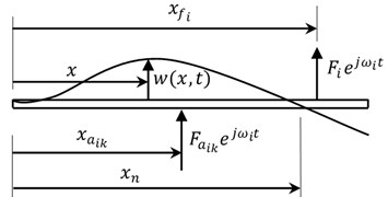
It is assumed that nodes are required to be enforced at certain locations on the beam structure using the applied control forces given by:
where and are the amplitude and location of the th applied control force. In general, a total of applied control forces are required for enforcing nodes on a beam structure that is excited by harmonic forces [8, 9].
In order to calculate the control forces amplitudes, the equation of motion is derived first using Hamilton’s principle. The kinetic energy of the beam system can be written as:
where is the beam material density in kg/m3, is the beam cross sectional area in m2, is the beam transverse deflection in m, and is the time in s. The potential energy can be written as:
where is the beam material modulus of elasticity, in N/m2, and is the moment of inertia of the beam cross sectional area, in m4. The virtual work done by the external nonconservative forces can be expressed as:
where represents the damping forces, given by:
Two types of damping are included in Eq. (6), the viscous type having coefficient and the viscoelastic type having coefficient .
The equation of motion can be derived by applying Hamilton’s principle, given by:
after substituting Eq. (3-6) and performing the variational mathematics with integration by parts, the following equation of motion can be obtained:
It is noted that, since damping exists, complex exponential functions are used in the representation of the excitation and applied control forces leading to simpler mathematical manipulations. Consequently, it assumed that the input forces are given by their real parts which results in the real part of the beam deflection.
3. Problem formulation
In this section, Green’s function is utilized to derive the exact algebraic equation for calculating the steady-state beam deflection. Since the beam system is assumed to be linear, the superposition principle applies and the solution of Eq. (8) is assumed to have the following form:
where is the steady-state deflection amplitude of the beam at location due to harmonic excitation and control forces. Consequently, the system will execute a simple harmonic motion with the same response frequency as the driving frequency.
Substituting Eq. (9) into Eq. (8) results in:
Once again, and by virtue of the superposition principle, Eq. (10) reveals that the governing equation for the steady-state response due to each harmonic excitation force can be considered separately as:
Therefore, the design of the applied control force(s) and the resulting steady-state response can be calculated separately for each excitation force and then combined, using Eq. (9), to obtain the total steady-state response due to the total number of distinct harmonic excitations.
At this stage, it is convenient to work with dimensionless quantities so that the analysis becomes more general. Therefore, the following dimensionless variables and coefficients are defined:
where:
The resulting dimensionless form of Eq. (11) becomes:
where a prime denotes differentiation with respect to and .
Before proceeding with the solution of Eq. (14), the caret on the dimensionless quantities is dropped for the sake of convenience. The solution of Eq. (14) is sought by utilizing the dynamic Green’s function. Hence, if the dynamic Green’s function, denoted by , is obtained from the solution of the following differential equation [10]:
then the solution of Eq. (14) is given by the following integral form:
where is given by:
The Green’s function, , for the beam is defined as the response at position due to a unit concentrated force applied at position . Utilizing the properties of the Dirac Delta function, the integration in Eq. (16) can be carried out to give:
Eq. (18) is an algebraic equation that provides the exact closed form solution for the beam steady-state deflection amplitude at any location resulting from the application of the excitation and control forces.
From Eq. (15 and 17), it is observed that Green’s function varies with the excitation frequency among other parameters. Furthermore, Green’s function value becomes complex if either the beam external damping or internal damping is present.
Several researchers have reported the solution of Eq. (15) (see, for example, Refs. [10] and [11]) for different beam boundary conditions.
4. Enforcing a node
The derivations for the analytical solution of the applied control force that results in creating a point, at location , on a beam having zero deflection, called a node, is presented in this section. One control force is required to enforce the node that can be calculated using Eq. (18). First, the deflection at location is substituted in Eq. (18) to obtain:
To create a stationary point at location on the beam, the right hand side of Eq. (19) is set to zero, which can be satisfied when:
As seen in Eq. (20), the calculation of the amplitude of the th applied control force to enforce a node on the beam that is vibrating as a result of the application of the excitation force having amplitude and frequency is very simple, exact, and straightforward. Next, the calculations for the amplitudes of the other excitation frequencies to enforce a node on the same location are performed separately. Finally, the steady-state deflection can be calculated using Eq. (18) and the total response is obtained using Eq. (9).
5. Enforcing a robust node
In many applications, the excitation frequency value may not be exactly known or has a tendency to drift with time. In this case, it is desirable to design control forces to enforce robust nodes that are insensitive to excitation frequency variations within a desired range. This is performed by adding a constraint that forces the derivative of the steady-state deflection amplitude at the node location to zero. Therefore, a second control force is required to achieve the objectives of enforcing the node in addition to imposing the frequency derivative constraint. The steady-state deflection amplitude at the node location with two control forces, using Eq. (18), is given by:
The derivative of the steady-state deflection at the node location with respect to the excitation frequency can be expressed by:
where the coefficients and are defined as:
It is noted that the differentiation of the Green’s function can be performed easily because Green’s function derivation results in exact algebraic equation that is explicit function of excitation frequency and other parameters. Setting Eqs. (21-22) to zeros results in two linear equations that can be solved for the two control forces amplitudes.
6. Simulations and discussions
In this section, numerical experiments are performed using the procedure outlined in the previous sections to create a node in a vibrating beam. The outlined numerical method is applied on simply supported and cantilever beams, although the method is applicable to beams having any end supports.
It is to be noted that all the parameters and variables used in the following examples are dimensionless, which are defined in Eqs. (12-13). These parameters can be easily transformed to their dimensional counterpart once all the parameters of the beam structure are defined. Consequently, all the parameters stated in the following examples are shown without dimensions.
The first numerical example considered is to apply the numerical procedure on a uniform damped simply supported beam of length excited by two concentrated harmonic forces of amplitude , excitation frequencies and , and location . The coefficients of external damping is while that for the internal damping is 0.001. It is desired to impose a node at the location using one collocated control force for each excitation frequency, i.e., . The calculated applied control forces amplitudes are equal to –1.712 and 1.226 for the first and second excitation frequencies, respectively. The resulting steady-state deflections of the beam for the uncontrolled case (red dashed line) and one node case (blue solid line) are shown in Fig. 2. As seen in the figure, a node at exactly is created for both deflections resulting from the two excitation forces.
Fig. 2The steady-state deflection for the uncontrolled case (red dashed line) and one node case (blue solid line) of a damped simply supported beam when ω1= 10, ω2= 85, xif= 0.5, xn= 0.8, xa11=xa21= 0.8
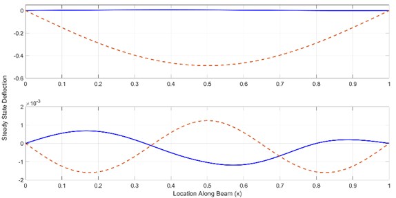
Table 1Deflection amplitudes at the node location for the non-robust and robust cases
Case No. | Frequency | Steady-state deflection amplitude at node location () | |
Non-Robust | Robust | ||
1 | 30 | 0 | 0 |
2 | 31 | –3.2778×10-04 | 3.4805×10-06 |
3 | 32 | –5.8178×10-04 | 1.1922×10-05 |
4 | 33 | –7.8467×10-04 | 2.3246×10-05 |
5 | 34 | –9.5136×10-04 | 3.6173×10-05 |
6 | 35 | –0.0011 | 4.9900×10-05 |
7 | 36 | –0.0012 | 6.3913×10-05 |
8 | 37 | –0.0013 | 7.7882×10-05 |
9 | 38 | –0.0014 | 9.1597×10-05 |
10 | 39 | –0.0015 | 1.0492×10-05 |
Fig. 3The steady-state deflection for the non-robust (top) and robust (bottom) control force(s) design for a damped cantilever beam with ω= 30, xf= 0.76, xn= 1, xa1 = 1, xa2= 0.9
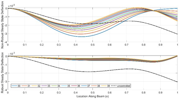
The second example shows the effectiveness of the robust control force design with respect to excitation frequency variations. The numerical procedure is applied on a damped cantilever beam with length subjected to excitation forces at with a frequency . The coefficients of external damping is while that for the internal damping is . A robust node is desired at using two control forces at locations and . The solution of this case is compared with the non-robust design, outlined in Section (4), having the following parameters: 1, 0.1, 0.001, 30, 0.76, 1, and . The calculated steady-state deflections for the robust and non-robust cases when the excitation frequency varies between 30 to 39 is shown in Fig. 3. Furthermore, the values of the deflection amplitudes when the excitation frequency varies between 30 to 39 for the robust and non-robust cases are shown in Table 1. It is clear from the Fig. 3 and Table 1, that the robust control design has reduced the effect of changing the excitation frequency on the steady-state deflection not only at the node location but also along the whole beam span compared with that for the non-robust case.
7. Conclusions
In this paper, Green’s function is utilized to develop an exact analytical solution for the control forces required to impose points with zero deflection, called a node, on a beam structure excited by disturbances having multiple frequencies. The principle of superposition allows the numerical procedure to be applied for each excitation force independently, which greatly simplifies the computations for the designed control forces. In general, each node requires a control force to be applied at specified location on a beam. The resulting equations for the control forces are linear algebraic equations which can be solved using Gauss elimination. Furthermore, the derived analytical equations are utilized to calculate the control forces amplitudes that result in enforcing a robust node that have minimum sensitivity to excitation frequency variations. The validity of the numerical technique is demonstrated by numerical examples that shows its effectiveness in controlling and reducing the vibrations not only at the desired points but also along regions and may be the complete beam span.
References
-
Korenev B. G., Reznikov L. M. Dynamic Vibration Absorbers: Theory and Technical Applications. John Wiley, New York, 1993.
-
Cha P. D., Pierre C. Imposing nodes to the normal modes of a linear elastic structure. Journal of Sound and Vibration, Vol. 219, 1999, p. 669-687.
-
Alsaif K., Foda M. A. Vibration suppression of a beam structure by intermediate masses and springs. Journal of Sound and Vibration, Vol. 256, 2002, p. 629-645.
-
Foda M. A., Albassam B. A. Vibration confinement in a general beam structure during harmonic excitation. Journal of Sound and Vibration, Vol. 295, 2006, p. 491-517.
-
Foda M. A., Alsaif K. Control of lateral vibrations and slopes at desired locations along vibrating beams. Journal of Vibration and Control, Vol. 15, 2009, p. 1649-1678.
-
Bassam Albassam A. Creating nodes at selected locations in a harmonically excited structure using feedback control and Green’s function. Shock and Vibration, Vol. 2019, 2019, p. 3261628.
-
Cha P. D. Enforcing nodes at required locations in a harmonically excited structure using simple oscillators. Journal of Sound and Vibration, Vol. 279, 2005, p. 799-816.
-
Cha P. D., Ren G. Inverse Problem of imposing node to suppress vibration for a structure subjected to multiple harmonic excitations. Journal of Sound and Vibration, Vol. 290, 2006, p. 425-447.
-
Cha P. D., Buyco K. An efficient method for tuning oscillator parameters in order to impose nodes on a linear structure excited by multiple harmonics. Journal of Vibration and Acoustics, Vol. 137, Issue 3, 2015, p. 03101.
-
Roach G. F. Green’s Functions: Introductory Theory with Applications. Van Nostrand Reinhold Company, London, UK, 1970.
-
Roach G. F. Greens Functions. Cambridge University Press, Cambridge, 1982.
About this article

